2 Data Structures and Processing Paradigms

This chapter discusses the most commonly used data structures and general problem solving strategies for natural language processing (NLP). Many data structures of NLP reflect the structure of language itself. Language in use has both a sequential order and a hierarchical structure.  Thus, data structures such as strings, lists, trees, and graphs are commonly used.  Other essential data structures for NLP reflect the processes of statistical machine learning and data science, where vectors and their generalizations, called tensors, are used for representing associations between entities and values, such as probability distributions over   categories.

The main processing paradigms for NLP are search and classification. The search methods all derive from techniques for searching graphs that are common across computing, such as breadth-first and depth-first search. NLP also makes use of AI-specific techniques that aim to make the search more efficient by modifying the order of the traversal.  As an abstract process,  search is a method for addressing questions, where we do not have a set of candidate answers, such as finding out  how a sentence can be derived from a set of rules. By contrast, classification is a method for addressing  questions, where we do  have a set of candidate answers.  We call the systems that select or rank the answers “classifiers”.  There is a search process, but it usually only occurs when we build the classifier, rather than when it is used. However, some implementations of classifiers first create a probability distribution over the candidate answers and then use search as a final step to find the best one.

The construction of modern classifiers uses machine learning. Machine learning  systems take minimally processed data as input and  iteratively adjust the values of internal parameters, to build models that optimize some function, such as minimizing the error over some set where the answer for each is known.  This phase is called training. It is a  type of search where each step involves increasing or decreasing the value of numeric variables and evaluating the impact on the error measure. Training often takes a long time, (and a large amount of data) to create an accurate model,  but during use classifiers are very fast – and robust because they always provide an answer. However,  when  a problem is new, training data may not yet exist,  so we may start with a search-based method.

We will start by discussing data structures and then two processing paradigms and their application to NLP.  We will also take a more in-depth look at machine learning, since it plays such an important role in current implementations of NLP.

2.1 The Data Structures for Natural Language Processing

The data structures most common to NLP are strings, lists, vectors,  trees, and graphs.  All of these are types of sequences,  which are ordered collections of elements. Unprocessed data is usually input as string data which are processed into lists or vectors, representing individual words, before subsequent processing in the NLP  pipeline. This processed data is usually not just a list or vector of strings, but sequences of complex objects that keep track of various attributes associated with each token, such as part of speech. Later stages may add additional annotations, such as marking the beginnings and endings of  important sequences within a sentence, such as the names of entities. This section will overview the most commonly used data types along with examples of their application in NLP.

2.1.1 Strings

Strings are sequences of characters. They are the primary way that unprocessed text data is represented in NLP systems. One string may be used to hold an entire document, a line of a text file, a sentence, or a single word. Important operations for strings include concatenation (creating a string by sequentially combining two input strings into one), matching substrings (e.g., to check for a prefix or suffix), and finding the length of a string (e.g., strings that are very short might be abbreviations). Specifying patterns within strings, such as punctuation or word endings, is usually done by means of strings of text that allow one to name specific characters, possible ranges of characters (such as [a-z]), and how often they occur (e.g., once, zero or more, or one or more times). These formatted strings are called regular expressions and have been in use since the 1940’s but have become more standardized over time, such as the POSIX Basic Regular Expression (BRE) format.^[1][2]

Today, most programming languages (e.g. C++, Python, and Java) have functions for handling regular expressions^[3]. They also have mechanisms for specifying substrings (slicing) or particular ranges of characters within a string. When input to an NLP system is provided as a string, the first thing the system will need to do is separate the string into separate words and sentences. This step is called tokenization. The general idea is to  use whitespace as a delimiter, but the task must also consider special cases, such as contractions and quoted speech. Software libraries for NLP, such as spaCy and  the Natural Language Toolkit (NLTK),  include prebuilt functions for tokenizing sentences. NLTK includes five different options, each of which provides slightly different results.^[4] Sometimes, getting tokenization right requires using hand-built patterns, because people will differ in punctuation habits, such as placing quote marks or parentheses inside or outside end-of-sentence punctuation.

2.1.2 Lists

Lists and vectors are both ordered collection of elements.  Lists are used to hold sequences where the sizes of elements might vary, such as sequences of words. Lists can also have more or less elements over time.  (Lists that are immutable during the execution of a program are sometimes called tuples.) Some programming languages allow direct access to elements of a list using an index, while some may only allow iterating through them sequentially from the front. Lists (and more generally sequences) are often used as the representation format for sharing results between different stages of an NLP pipeline; for example each element corresponds to all the information about a particular token in the order in which it occurred in the original input.

Important operations over lists include being able to find individual elements or patterns of elements within the list.  Patterns over elements of a list can make use of regular expressions for looking within a single token or a list of tokens. For example, the spaCy toolkit has a function called “matcher” that finds sequences that match a user defined pattern^[5]. These patterns can match a variety of word attributes, including the word type (lemma) or the part of speech.   Figure 2.1 shows some example patterns for spaCy and phrases they would match. Addition examples can be tested using an online pattern tester provided by Explosion.ai^[6]

[{"TEXT": {"REGEX": "^[Uu](\.?|nited)$"}},
 {"TEXT": {"REGEX": "^[Ss](\.?|tates)$"}},
 {"LOWER": "president"}]

[{"ORTH": "("}, {"SHAPE": "ddd"}, {"ORTH": ")"}, 
 {"SHAPE": "ddd"},{"ORTH": "-", "OP": "?"}, 
 {"SHAPE": "dddd"}]

[{'LIKE_NUM': True, 'OP': '?'},
 {'POS': 'ADJ', 'OP': '?'}, 
 {'LEMMA': 'duck', 'POS': 'NOUN'}]           

Note that the most common sequences of language will be determined by the syntax, or grammar, for that language. Deriving the syntactic structure of a sentence for a particular grammar using an algorithm is called parsing. Syntax for English will be discussed in detail in Chapter 3 of this book. Parsing will be discussed in Chapter 4.

2.1.3 Vectors

Vectors hold elements of the same size, such as numbers, and are of fixed size. They are one-dimensional, which means elements can be accessed using a single integer index. Similar representations of higher dimension are given special names; a matrix is a two-dimensional, rectangular structure arranged in rows and columns. The term tensor is used to describe generalizations of matrices to N-dimensional space.^[7]  Important operations for vectors include accessing the value of an element of the vector, finding the length of a vector, calculating the similarity between two vectors, and  taking the average of multiple vectors.

For much of data science, including modern NLP, vectors are used as a representation format for a variety of tasks.  For example, vectors can represent subsets of words or labels from a fixed vocabulary.  To do this, each element corresponds to a single word in the vocabulary and the value is either one or zero to indicate whether or not the word is included in the set. Vectors where only a single element can be zero^[8] are often used as an output format (to indicate the selected class label or type of word in context– e.g. to discriminate between a noun versus verb sense.) Vector elements can also capture a  probability distribution over a set, where the value of each element corresponds to the probability of that element, a value between 0 and 1, and the sum across all such values is 1. Calculating such a probability distribution is often done using a  “softmax” function, which is a mapping from a vector of real numbers, onto a probability distribution with the same number of elements, where the probabilities are  proportional to the exponentials of the input values. Two applications of vectors are of special note here: the use of vectors to represent documents for information retrieval (which has been termed the “Vector Space Model”) and the use of vectors for word embeddings which are a  representation of the meaning of words, which can also be generalized to represent longer phrases and sentences.

2.1.3.1 The Vector Space Model for Information Retrieval

The Vector Space Model (VSM) ^[9] was introduced for automated information retrieval. In the VSM, the elements of the vector correspond to words in a vocabulary and the value is a weighted measure that combines the frequency of a term (word type) within a document with a measure of its frequency across a set of documents. The VSM draws on the insight that the importance of a word  in a document is directly proportional to the number of times it appears in a document,  but inversely proportional to the number of  documents in which it appears^[10].  The combined measure is called “term frequency-inverse document frequency” (tf-idf).  In this context, term frequency is the raw count of the term in a document divided by the total number of words in the document. Inverse document frequency  is most commonly calculated as the log of the quotient of the total number of documents in the corpus divided by the number of documents that contain the term. The log is used to prevent  calculation errors caused by numbers that are too small (called underflow). Variations of these measures are sometimes used to address data sparsity (called smoothing) or to prevent bias towards longer documents (normalization).

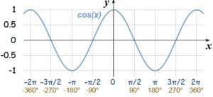
Using this model, the similarity between documents (or between a query and a document) can be determined using  cosine distance, which measures the angle between two vectors. Figure 2.2 shows the formula for cosine distance,  a graph of it as a function, and a visualization of the angle measured^[11]. What makes cosine good for measuring similarity is that this function ranges between zero and one, reaching it maximum only when the two vectors line up exactly. Cosine similarity is also used  to assess semantic similarity in other applications including when vectors  are used to represent the meaning of words, phrases or sentences, where they are called “embeddings”. Embeddings are the topic of the next subsection.

Figure 2.2  Calculation and visualization of cosine similarity of two vectors

Calculation of  cosine between A and B and       a graph of the cosine function	Illustration of cosine

2.1.3.2 Word Embeddings

Vectors are commonly used to represent meanings of words. These vector representations are called word embeddings. Embeddings differ from document vectors in that the components of word embeddings might not correspond to anything in the real world.  Instead, these vectors organize words into a kind of continuous thesaurus or hash table, giving each word type a unique vector of numbers that allows us to tell words apart and also to measure their similarity (such as by the cosine measure discussed in the previous section). This idea has been explored most directly in an approach called hash embeddings^[12].

Vectors are created through an optimization process where the objective is to minimize the error for some measurable  task or set of tasks. The optimal value is found by searching; the method used is typically  a stochastic approximation of gradient descent. (We will discuss gradient descent in a later section of this chapter). When pretrained embeddings are used it is important to use the embeddings that were trained on data most like what is anticipated in the target application. Well-known approaches  to creating word embeddings include: Word2vec,  GloVe, and Elmo, which we overview here.

Word2vec^[13] converts a corpus of words into numerical vectors using local statistics; it can either use context (e.g., a  fixed number of words on either side) to predict a target word (a method known as continuous bag of words), or use a word to predict a target context, which is called a skip-gram. Two variations of Word2vec are available:  one that works better on high frequency words and one that works better on low frequency words. For high frequency words, an approach called “negative sampling” is used to maximize the probability of a word and context being in the corpus data if it is, and maximize the probability of a word and context not being in the corpus data, if it is not. Finding these optimal values can take a very long time.  For low frequency words, which require higher dimensionality vectors, a more efficient approach called hierarchical softmax can be selected. It uses a binary tree representation that reduces the computational complexity to O(log₂ |V|) instead of O(|V|), where |V| is the size of the vocabulary.

GloVe vectors^{[14] [15]} use global statistics to predict the probability of word j appearing in the context of word i with a least-squares objective.  The general idea is to first count for all pairs of words their co-occurrence, then find values such that for each pair of word vectors, their dot product equals the logarithm of the words’ probability of co-occurrence.

Elmo (Embeddings from Language Models)  vectors^[16] contain values that have been learned from a neural network with a particular architecture known as a bidirectional Long Short Term Memory  (biLSTM or biLM) network.  These networks have multiple internal layers, some of which provide feedback to each other. Bidirectionality refers to training on both the original sentences and its reverse to captures certain syntactic dependencies on the semantics of a word.  In addition, unlike the other types of vectors discussed here, the representation of a word using an Elmo vector is a function of the entire sentence in which it occurs, rather than just a small number of nearby words.

For a particular application, the method of training is likely to not be as important as the data that was used to create the vectors, which should be as similar to the target domain as possible. There are pretrained vectors  available for several common domains. A common source of  pretrained embeddings is the Stanford Natural Language Group^[17]. There are also programs (with detailed instructions) that are available to train new vectors from a corpus. Software for training on new data can be found within open source and commercial (but free) software libraries, including  Rehurek’s Gensim^[18] and Fast Text^[19]. The spaCy library ^[20] also includes pretrained embeddings within the larger versions of their language models. The domains commonly used for pretraining are: Wikipedia (a web-based encyclopedia), Gigaword (newspaper text,  including  Associated Press and New York Times), Common Crawl  (web page text), Twitter (online news and social networking text), Google News  (aggregated newspaper text), and  the “1 Billion Word Benchmark”, approximately 800M tokens of news crawl data first distributed at a machine translation conference (WMT) in 2011.  These pretrained vectors cover vocabularies of 400K to 2.2M words, with vectors of dimension from 50 to 300.

2.1.4 Trees and Graphs

When one considers the organization of an entire sentence, or processing architectures for finding such organization, NLP algorithms rely on the datatypes of trees and graphs. Graphs are specified by a set of nodes and connections between pairs of nodes, called edges.  Trees  are a special case of graphs where edges are directed edges and each node has a unique predecessor (the parent) and multiple possible successors (the children).  By convention the root (a node with no predecessor in the tree) is drawn at the top. For NLP, data is most likely to be represented as a tree.  Graphs are used as a processing model as a way of representing the state of a search or the architecture used to train a classifier.

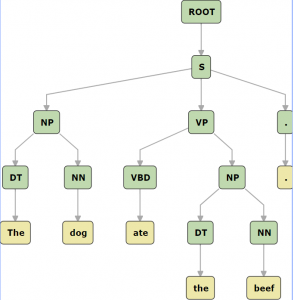
Trees are used to represent the syntactic structure of sentences, because sentence structure includes relations among words and phrases  that may be nested, and each sentence has a unique head. (The head of a sentence is usually given as the main verb of the main clause.)  Consider the sentence, “The dog ate the beef.”  In this sentence (S), “ate” is the main verb (VBD).  The sentence has two noun phrases (NP) nested inside it:   “the dog” and “the beef”.  These noun phrases (NP) both contain a determiner (DT) and a noun (NN). Figure 2.3 shows what this would look like drawn as a tree, using the symbols from a typical grammar.

Figure 2.3 Example phrase structure parse tree (Image from Stanford CoreNLP.run)

There is a direct correspondence between nested lists and trees, so both can be used  to represent syntactic structures of sentence. The structure for the sentence shown in Figure 2.3  is the same as the following nested list:

(S (NP (DT the) (NN dog))
(VP (VBD ate) (NP (DT the) (NN beef))))

We can also capture this  information as a list of subsequences (called spans), as in the following:

[(DT, the, 0, 1), (NN, dog, 1, 2), (VBD, ate, 2,3),(DT, the, 3, 4), (NN,  beef, 4, 5), (NP, 0, 2), (NP, 3,5), (VP, 2, 5), (S, 0, 5)]

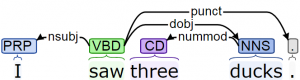
The type of grammar in this example is called a phrase structure grammar. Other approaches to syntax focus on binary relations, or dependencies among the words in a sentence. Figure 2.4 shows a dependency parse of the sentence “I saw three ducks” (which has been analyzed to include four dependencies: I is the nominal subject of saw; three is a number modifier of ducks; ducks is a direct object of saw; and the period is a punctuation mark).

Figure 2.4  Example dependency structure parse tree (Image from Stanford Corenlp.run)

Graphs are more general that trees, because they allow nodes to have multiple incoming edges. While they are not needed to represent sentence structure, they are helpful in describing how language is processed.  Graphs  form the basis of the processing architectures for both search based parsing and analysis using neural networks. In a search, the nodes of the graph  correspond to a machine state and possible alternative next states.  In a neural network, the nodes of a graph correspond to operations or functions, which can have any number of inputs and outputs. The edges of a neural network, which represent the data that flows from the output of one node to the input of another are tensors, as they may be scalars, vectors, matrices, or higher-dimensionality structures. In both search graphs and neural network, the nodes and edges represent models of process rather than data.

This concludes our introduction to the data structures of NLP. We will next consider the two primary processing paradigms: search and classification.

2.2 Processing Paradigms for Natural Language Processing

NLP is an instance of Artificial Intelligence (AI) problem solving. AI methods for NLP include search and classification. Search is used when we do not have a ready set of answers or we are interested in the derivation of a solution, that is, the steps involved in reaching it. Search has a variety of uses for NLP, but has been most closely associated with rule-based parsing.  In a search,  at each step, what happens next, is determined from a combination of stored knowledge and current inputs. Often, there may be more than one rule or function that applies with different outcomes depending on which one is applied. When this happens, different alternatives are considered as part of a search process, with the search terminating when either the desired outcomes are achieved or it is determined that a solution is not possible.  Classification involves labeling observations with one of a known set of categories. This labeling can be done by either rule-based matching or by applying a classifier that has been created using statistical machine learning. This section will consider both general paradigms. In the next section we will  overview how statistical classifiers are created.

2.2.1 The Paradigm of Search

The general type of search used in AI is called state space search. Such searches are specified by providing a specification of the initial conditions, a specification of the termination condition, and a specification of methods that manifest a transition from a given set of conditions (or “state”) to another. An AI search space may be only implicit; nodes may be generated incrementally. States may be explored immediately or stored in a data structure for future exploration. After being explored, states may be discarded, if they are not part of the solution itself. Sometimes the solution is the goal state – to answer a “yes-no” or “what” question – but sometimes the solution is the path – to answer a “how” question, such as “how is a sentence derivable from a given set of rules that constitute a grammar”.

State space search is a generalization of algorithms for traversing tree and graph data structures, including breadth-first search, which expands all nodes adjacent to the current node before exploring further nodes, and depth-first search, which expands one node adjacent to the current node and then makes that node the current one, expanding along a single path from the root. Another type of search is known as best-first search. A best-first search chooses what node to expand on the basis of a scoring function. For example, a scoring function might favor nodes believed closest to  the goal, which is known as a “greedy” search. Or, the function might  try to balance the accumulated cost of getting to a node with the estimated distance to the goal, as in A* search. Another useful best-first search is beam search, where the number of states kept for future consideration is bounded by a fixed number, called the “width” of the beam. (This list of search strategies is not exhaustive, but covers the primary ones that have been used for NLP.)

Search algorithms are used in NLP for identifying sequences of characters within words, such as prefixes or suffixes. They have also been used for parsing, to find sequences of words that correspond to different types of phrases, where these patterns have been described using rules. These rules can specify simple linear sequences of types that are mandatory, optional or can have specified number of occurrences (e.g. zero, zero or more, one, one or more), or can specify arbitrarily nested sequences, as with a context free grammar. For parsing, Beam search has been used to limit the number of alternatives that are kept for consideration when there are a large number of rules that might be applicable.  Beam search has also been used as a way of finding the best possible sequence given the results of a machine learning algorithm designed to provide a probability distribution over each word in the vocabulary for each word in an output sequence. This type of algorithm, known as an encoder-decoder, is now commonly used for generating text, such as for creating captions or brief summaries.

Hill-climbing search and its variants use a function to rank the children of a current node to find a node that is better than the current one, and then transitions to that state, without keeping any representation of the overall search path.  Gradient descent is a variant of hill climbing that searches for the child with minimum value of its ranking function. For machine learning, this type of search is used to adjust parameters to find the minimum amount of error or loss in comparison to the goal by making changes proportional to the negative gradient, which is the multivariate generalization of a derivative (akin to the slope of a line). Hill-climbing and gradient searching do not backtrack, and hence do not require any memory to track previously visited states.

2.2.2 The Paradigm of Classification

A classifier is a function that takes an object represented as a set of features and selects a label for that object (or provides a ranking among possible labels). The first classifiers were given as a set of rules. These rules were hand-written patterns (e.g., regular expressions) for assigning a label to an object. Rules for NLP often name specific tokens, their attributes, or their syntactic types. Examples of patterns are shown in Figure 2.1, in the section that discusses lists. Statistical classifiers select or rank classes using an algorithmically generated  function called a language model that provides a  probability estimate  for sequences of items from a given vocabulary. Language models can contain varying amounts of information. A small, simple model might only have information about short sequences of words and the correlation between those sequences and sequences of labels (such as parts of speech or entity types), while a more complex model might also include meaning representations, called embeddings, that were discussed as an example of vectors.

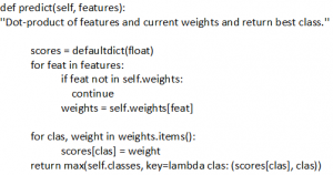
Statistical classifiers can be designed to either pick the single best class or to provide a ranked list of possible classes along with a score of their certainty or estimated probability of being the correct class. One example of a single-best classifier is a Perceptron Classifier, which represents both the input features and model weights as vectors, computes their dot product (which is a sum of the products of the corresponding entries of the two vectors) and returns the one with highest value. Figure 2.5 shows the pseudocode for a perceptron classifier. (The training of a perceptron will determine the value of the weights.)

Figure:  2.5  Pseudocode for a Perceptron classifier

Today, most classifiers are created via supervised machine learning.  Supervised Machine Learning (SML) is a method of creating a function for combining the contributions of different features of the input to select an output class that will best match the output classification given to similar examples from the training data. SML models are trained using data sets of instances where the correct class has been provided, either by asking people to annotate the data based on a guideline, or by using some aspect of the data itself, such as a star rating, as the class.

Classification as an approach has become increasingly important as many NLP tasks can be mapped to classification tasks, given the right representation. For example, the task of recognizing named entities within a sentence and labelling them with their type, such as PERSON (PER) or LOCATION (LOC) can be cast as a classification task using an encoding called IOB, which stands for “inside” “outside”  “beginning”, to classify each word in the entity sequence. Words marked with tags with the prefix “B” are the first word in the sequence. Words marked with tags with the prefix “I” are “inside” the sequence.  All other words are “outside” which means that they are not part of any recognized entity. After a named entity classifier is used, another process can traverse the classified tokens to merge the tokens into objects for each entity.  Figure 2.6 includes an example of IOB encoding for named entity recognition.

The same approach can be used for the task of marking the noun phrases within a sentence. Figure 2.7 shows an example of an IOB encoding for bracketing noun phrases^[21].

Classification can be applied to units of different sizes (e.g. words or complete sentences) and can be applied either to each input unit independently, or performed to optimize over a sequence of units (called sequence modelling). For example, we might want to classify all elements of a sequence of words in a phrase at the same time. Examples of methods used for sequence modelling include Conditional Random Fields, Hidden Markov Models, and neural networks. A simple neural model that has been used effectively for some  NLP tasks is the Averaged Perceptron.  Another alternative is to classify sequences using a structured output label (such as a parse tree) rather than a discrete symbol or an unordered set of symbols. Structured modelling can be more accurate than either word-level modelling or sequence modeling, however obtaining training data with structured labels is harder, and would require a much more complex type of neural network, involving multiple layers.  More information about machine learning, and its use in training classifiers, will be discussed in the next section.

2.3 Overview of Machine Learning

Approaches for learning models based on machine learning have their origins in  search, where the goal of the search is to find a function that will optimize the performance of the system. The term “machine learning” was first coined by Arthur Samuel in the 1950’s to describe his method for developing a program to play the board game  of checkers.  His game player selected the correct move for each turn based on a function that combined the contributions from features such as piece position and material advantage. This function was trained  by adjusting the coefficients of a linear polynomial to favor “book moves” (a type of supervised learning) and moves that increased the average number of wins over repeated games against itself. Today we would call such an approach reinforcement learning or semi-supervised machine learning. Thus, although ML classifiers do not search during the classification process itself – it is more like table lookup or hashing – the training algorithms for machine learning do use search to create the functions that combine the contributions of different features. A common type of search used in machine learning algorithms is gradient descent, as they try to minimize the amount of error or “loss” between the output value of the system and the true value, based on the data.

Samuel’s approach introduced several ideas that are still used among all machine learning methods today: algorithms learn models for making a decision about what to do (or how to label something) based on a set of observations, each of which is represented as a finite number of attributes (also called features). These features may correspond to an unordered set, or they may represent a sequence. The algorithms all have some training objective which can be internal (e.g., minimize the amount of error on training data) or external (e.g., maximize the number of games to be won when the model used in simulated play). The algorithms “train” by changing the values of internal parameters, such as coefficients of scoring functions over several iterations until they converge at an optimal configuration (or some fixed maximum determined externally).

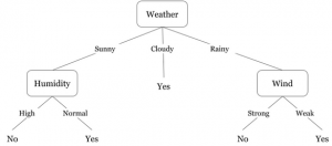
A machine learning approach that has a long history, and is still used today, is decision tree learning (such as ID3, C4.5, J48, Random Forest, etc.). A decision tree is a tree where each node represents a test on one of a fixed set attributes of the input. Each edge out of a node represents one possible outcome for the test, like the different branches in a case statement (or switch) in a programming language. For example, a binary test has two branches one for true and one for false.  Figure 2.8 shows a decision about whether the weather is comfortable for being outside, which can be yes or no.  The tree considers  three attributes of the input: the wind (which can be strong or weak), humidity (which can be high or normal), and weather (which can be sunny, cloudy, or rainy). The paths through a tree correspond to rules that can be used to classify examples, with the leaves indicating the value of the class variable. Thus, any input whose value for weather is cloudy would be classified as yes (a comfortable day to be outside).

Figure 2.8 Example of a decision tree

Over a set of  attributes, many different decision trees are possible, but there are a small number of optimal trees that minimize the number of tests that must be performed. The trees can be learned from labelled examples by searching through the space of all possible trees by doing a greedy best-first search that picks the best attribute at each step and terminates when either all remaining examples fall within a single branch or all attributes have been tested.  It has been shown that the “best” attribute to test at a given node in the tree is the one that best splits subset of examples that match a particular path in a decision tree. The best split is determined by some function, such as information gain^[22]. One advantage of decision tree learning is that it provides easily extractable information about the importance of each attribute in how examples are classified.

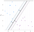
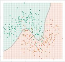
Today, there are many algorithms for training classifiers with labelled data.  The goal of all of them is to find decision boundaries between classes that will work well on both the training data and the future test data. For some problems, a linear boundary is sufficient (see Figure 2.9A) but for others, a nonlinear boundary is needed (see Figure 2.9B). Linear methods include decision tree learning algorithms, statistical approaches, like Naïve Bayes or Support Vector Machines,  and shallow neural networks, such as Perceptrons. Nonlinear boundaries can be found for clustering methods (such as K-nearest neighbors) and for neural networks that include multiple internal layers (Deep Learning).  Workbench tools such as Weka and WekaDeepLearning4J allow one to experiment with a variety of algorithms and visualize the results.

Figure 2.9 Examples of linearly and non-linearly separable data (images from Wikipedia)

A: Data that is linearly separable	B: Data that is non-linearly separable

In general, employing machine learning approaches is an iterative process of training and testing.  Training means running a learning algorithm on a data set where the correct class is provided to the algorithm so it can use the information to find values for internal parameters. Testing means applying the trained classifier to a subset of the data that was not used for training, but where the correct class is known. The performance of the classifier is then assessed. The most common measures to use are precision, recall, and F1. Precision is the proportion of correctly classified items of a given category among the total number of items it classified as the category. Recall is the proportion of correctly classified items among the total number of items that should have been classified as the category.  F1 is their harmonic mean  (which is calculated as two times the product of precision and recall divided by their sum).

Training and test sets can be created through a manual or  automated selection process. Manual selection, while less common, is sometimes done to assure consistency across training and testing over time. Manual selection risks biasing the results however. Instead, experimenters will  use N-fold cross-validation,  which is an iterative process where the data set is first partitioned into N equal subparts (the “folds”) and  then training is repeated N times, each time with a different one of the subparts held out as a test set. Afterward, the performance measures are averaged over all test sets.

The success of training classifiers (of all types) depends primarily on the data set available to train the model. (There can also be differences due to the training algorithm, so several are usually tried and compared.)  The data used for training should always be as similar as possible to the target test data and have enough positive and negative examples for each category, to minimize the impact of small differences in placement of boundaries. It is also important to choose an appropriate internal representation of the data as features.  A simple approach might consider each of the individual words – but this can be both too much and too little. The set of unique word types in any natural language is in the hundreds of thousands. One can reduce the number of features by using only the most important words for a corpus (e.g., using a tf-idf measure) or the most discriminative words for a classification problem (e.g., using a mutual information measure).  On the other hand, just using individual words may fail to discriminate among different senses of a word, so one may add bigrams (pairs of words) or part of speech bigrams (words with part of speech tags) or pretrained word embeddings  for each word in the input as features.

Training classifiers using neural networks  requires additional manual intervention. All versions of these algorithms are run repeatedly for a preset number of iterations (set by the experimenter) and make adjustments to the model of a fixed size, called the learning rate (also set by the experimenter) in the direction indicated by the objective function. Values set by the experimenter are called hyperparameters and generally they are set by a process of generate and test. For example, the experimenter tries different numbers of iterations to see what value provides the best performance. More is not always better, because running for too many iterations eventually leads to a problem called overfitting, which means that the model will not perform well on unseen examples. One approach to overfitting in neural networks is dropout^[23], which is where the inputs of some units are disabled randomly. Whether or not to use dropout is another user-settable parameter.

Neural networks also have a variety of architectures that can be configured. So-called “deep” neural networks are organized with several layers of different types of nodes.  See Figure 2.10 from Ruder(2018)^[24].

Figure 2.10 Example Deep Network architecture for NLP  (Image credit: Ruder, 2018)

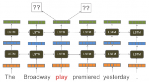Typically, as in the figure, the initial (bottom) layers are used to create a representation (encoding) of the input or to control the order in which the network will process an input that comprises sequence (such as a sentence or pair of sentences). Interior layers (called “hidden layers”) are used to change the dimensionality of the data (e.g., to match the input expected by the next layer) or to learn different substructures or dependencies among features of the input. The last (top) layers are used to create an output of the proper type. For example,  a softmax layer takes a vector of real-valued inputs and maps it onto a probability distribution, which is a value between 0 and 1.  The types of optimization functions used to update the nodes can vary;  common examples include Stochastic Gradient Descent and AdaDelta.

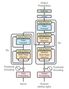
The first systems to use deep learning were built from separately trained, pipelined models of tasks such as labelling words with a part of speech (such as noun or verb) or labelling phrases with a semantic type, or a syntactic type or function (such as person, noun-phrase or noun-subject). However, the focus has been shifting towards creating networks that learn general models of language and work well for a variety of  tasks, from discriminating word senses to selecting the best answer to a question. These general networks often are built as  so-called “transformer” models,  such as  BERT, GPT-2 and XLNet, which are good for classification problems involving pairs of sequences. Transformers pair two general purpose subnetworks, an “encoder”, and a “decoder”. (See Figure 2.11 for an illustration.) The encoder is trained to model input sequences.  A decoder is trained to model output sequences.

An encoder may be trained to learn dependencies within the sequences by including layers of “self-attention” that take inputs from different positions within the sequence^[25]. A unidirectional model of attention uses the initial words in a sequence to predict later ones; a bidirectional model^[26], uses the words on either side to predict a left-out word, using an approach called “masking”, resembling the technique of cloze tests used for assessing reading comprehension^[27] or the assessment of age-related loss of hearing^[28] Decoders are trained to include attention to both the output of the encoder, sometimes called the “context vector”, and to dependencies within the output sequences.

Figure 2.11 Attention within Encoder and Decoder of a Transformer (Image credit: Vaswani et al, 2017)

Newer architectures for encoders, developed by Lee-Thorp et al (2021), replace multiple layers of self-attention with a single layer of linear transformations that “mixes” different input tokens, to create faster processing models; the group report that a “standard, unparameterized Fourier Transform achieves 92% of the accuracy of BERT on the GLUE benchmark, but pre-trains and runs up to seven times faster on GPUs and twice as fast on TPUs”^[29]. Other versions mix a single self-attention layer with Fourier transforms to get better accuracy, at a somewhat less performance benefit. Exploring such tradeoff is likely going to remain an active area of research for awhile.

Both encoder and decoders are trained on large collections of text, such as Gigaword^[30], which includes text from several international news services. Transformers for dialog must be trained on data collected from interactions between people, which can be gathered either by scraping portals where people interact (e.g.,  for language learners to practice conversation skills) or by creating tasks for pairs of crowd-workers. These datasets have then been annotated by researchers at universities or large companies, such as Google. Facebook research has assembled one of the most comprehensive collections of  openly available datasets and software tools, which they make available through its ParlAI project^[31].

For specific sequence to sequence classification tasks, the pretrained models are fine-tuned or updated with additional data from the target domain, such as pairs of questions and answers^[32]. The pairs of sequences can be given as two separate inputs, {S1, S2} or, more commonly, they are given as one concatenated input, by adding special tokens to indicate the start, separation, and end of each part of the pair, e.g., [Start]-[S1]-[Separator]-[S2]-[End]. These models have been shown to work fairly well for question answering, sentiment analysis, textual entailment and parsing^[33]. One limitation is that these models are big and slow in production – and thus cannot yet be used for real-time systems – however they could be used to create training data for simpler models.  Another concern has been that retraining such models consumes a huge amount of power; the carbon equivalent of BERT has been estimated  to be around the same a transatlantic flight^[34].

Workbench tools for deep learning include a growing number of preconfigured architectures and also support changing the values of the control parameters to assess their impact. Finding the best approach is an experimental process. When trying to solve a particular problem with these tools, a good way to start is to learn what algorithms and parameter values have been used most effectively in the past  for similar problems and then try to replicate the setup for one’s own data using a workbench tool.  There are also software libraries specifically for performing NLP using Deep Learning, some organized as notebooks, that can be used to perform experiments or build applications. Software from the start-up Hugging Face is most available, as currently it can be run either directly, within Google’s  “Colaboratory”, which includes notebooks for transformer-based NLP libraries using either TensorFlow 2 or PyTorch^[35], or from within spaCy, as “spacy-transformers”.

2.4 Summary

This chapter considered the most used data types and problem-solving strategies for natural language processing.  The data types include strings, lists, vectors, trees, and graphs.  Most of these are meant to capture sequences (e.g., of letters or words) and the hierarchical structures that emerge because of grammar. Feature structures or objects are needed to associate various attributes with tokens or types (as a way to keep the number of unique types of a manageable number). The processing paradigms of natural language processing include search, classification, and more generally, machine learning, where the development of a language model (including classifiers) using machine learning represents a complex combination of manual and automated search to find an optimal model for performing a given task. Many steps for these processing paradigms have been implemented in the form of software libraries and workbench style tools, however no tool exists that can predict the optimal approach or identify the most relevant data or the internal representation to use. For these tasks, understanding of language, including levels of abstraction, benchmark tasks, and important end-to-end applications, will be discussed in the remainder of this book.