4 Grammars and Syntactic Processing
If one wants to build systems that communicate with people in human language or that analyze people’s beliefs and behavior it is useful to perform a syntactic analysis of the text into either phrase or dependency structures first. The correct structures are specified using a grammar. Identifying the structure involves a variety of steps, that can be performed independently, in a sequence (which is known as a pipeline architecture) or can be learned as part of a complete language model trained using Deep Learning. Both NLP pipelines and Deep Learning models input unstructured text, as a file or stream of characters, and output either a single best analysis or a ranked set of alternatives. In between, they may include steps that assign part of speech tags to individual words, that group words into segments and provide labels to sequences of tagged segments.
Figure 4.1 shows a modern natural language processing pipeline. This pipeline is the one implemented in the NLP software library spaCy.
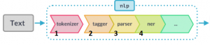 |
The steps associated with syntactic processing include tokenizing documents into individual sentences and words (1), followed by labelling words with syntactic categories (2), and identifying the syntactic structure that spans sequences of words, which is called parsing (3). These steps might be followed by a shallow analysis of meaning, such as named entity recognition (4), sentiment (not shown), or by a deeper analysis of semantic relations (not shown), which we will discuss in later chapters.
The pipeline processes of Figure 4.1 may be implemented as either search or classification (the processing paradigms we discussed in Chapter 2). Search-based parsing requires a computer-readable lexicon and grammar. The lexicon specifies the vocabulary, while the grammar describes constraints on the linear order of words and the sequences that correspond to well-formed constituents (phrases and clauses). Grammars and lexicons can be provided in a formal language, to be processed by a separate interpreter, or provided as functions in a programming language, that can be executed directly. Classification-based approaches require datasets annotated with the target structure that can be used for training. Widely used datasets for English include the Penn Treebank and OntoNotes for phrase-based annotations and the English Web Treebank (en-EWT)[1] for dependencies. These datasets have been used to create pretrained functions in software libraries such as NLTK, spaCy, Stanza, and UDPipe.
The remainder of this chapter will discuss pipeline processes 1 to 3 from Figure 4.1 (tokenization, tagging, and parsing).
4.1 Tokenization
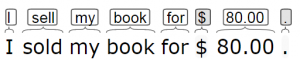
Tokenization divides a string into substrings and returns a set of tokens that represent the individual substrings. Simple tokenizers spit strings at whitespace (typically tabs and spaces) and create separate substrings for each punctuation symbol. More complex versions also find the root form (lemma) for each word, as shown in Figure 4.2, which shows how the tokenizer of Stanford’s CoreNLP system would split the string “I sold my book for $80.00.”
 |
NLP software libraries include predefined tokenizers and mechanisms for defining new ones. Figure 4.3 shows how tokenization can be called from NLTK and SpaCy in just a few lines of code. (The example is for processing the phrase “My pet cat.”) In some programming languages (e.g., Python) tokenizers can be implemented from scratch using built-in functions for splitting strings and regular expressions to find punctuation symbols or other characters, like “$”, in the spans between whitespace. More sophisticated tokenizers also create separate tokens for parts of a contraction (e.g., don’t is tokenized as {“do”, “not”}). Another system, the Wordpiece tokenizer (used by the BERT to create word vector representations[2][3]), splits unknown (out of vocabulary) words into substrings; for example “kindle” is split into [‘kind’, ‘##le’] and “recourse” is split into [‘rec’, ‘##ours’, ‘##e’]. The most sophisticated tokenizers (such as nltk.tokenize.punkt) have been trained on annotated data, such as the Penn Treebank, to identify strings that correspond to abbreviations, words that are at the start of a sentence (and hence can be safely changed to lower case), and collocations (or multiword expressions). Depending on the implementation, the result of tokenization may be just a list of strings or a list of objects with features set to capture the syntactic features and the canonical or dictionary form of the word (lemma) for spans that corresponds to words in a known vocabulary.
| Tagging in NLTK |
|
| Tagging in spaCy |
|
4.2 Part-of-Speech Tagging
Part-of-speech tagging takes a tokenized text and provides syntactic label for each token. Today, tags refers to either labels from the Penn Treebank II tagset (which is what NLTK uses) or tags from the Universal Dependencies tagset (which is what spaCy uses)[4]. Implementations of tagging use either hand-crafted rules, statistical modelling, or language modelling implemented with neural networks. Because part-of-speech tagging is such a common NLP task, prebuilt functions for tagging exist in major NLP software libraries, and can either be called individually (as in NLTK) or will be invoked as part of the standard NLP processing pipeline (as in spaCy). Figure 4.3 (in Section 4.1), shows example code for invoking the tagger within these two libraries, after sentences are tokenized.
The earliest successful taggers were rule-based or combined a rule-based approach with simple statistical modelling. Statistical taggers were first introduced by Marshall in 1983[5], but were not very accurate until larger and better datasets, such as the Penn Treebank, became available, so that more advanced modelling was feasible. The most successful taggers combine a wide range of information including the possible syntactic categories of nearby words, the overall probability associated with words being used a particular way (e.g., “eats” can be a noun or a verb, but it is more typically a verb), the probability of suffixes and prefixes being associated with different parts of speech (e.g., words that end in “-ly” are usually adverbs), and the capitalization of a word (e.g., words that begin with a capital letter are usually proper nouns). Rules for tagging can capture these known linguistic generalizations.
The simplest statistical models just use the most frequent category for each word. Sequence-based modelling (a type of sequence classification) involves finding the best sequence of tags for an entire sentence (rather than just a single word). These approaches can combine information about the most common category of a single word with those of nearby words, which is the approach taken by Hidden Markov Models. More advanced approaches, such as Maximum Entropy Markov Models (used by the Stanford CoreNLP tagger) and Averaged Perceptrons (a neural approach used in NLTK), consider the frequency of subsequences, as well as the other linguistic features, but adjust their impact by measuring the association between each feature and tag in a training corpus. Thus, sequence classification requires a data set of sentences where each word has been correctly tagged. Also, the corpus must be large enough so that the algorithm can find enough examples within the training corpus for the estimates to be meaningful. A third factor in the success of taggers trained from data is the similarity between the genre used for training and the genre of the target. Treebanks exist for newspaper text, as part of the Penn Treebank, and a variety of Web texts, such as blogs, as part of the English Web Tree Bank (a treebank created from Twitter posts as part of the CMU TweetNLP corpus), and a treebank created from GENIA, a collection of abstracts from the medical literature (which can be obtained from the Stanford NLP group[6]).
In sections that follow, we will consider rule-based, statistical, and neural approaches to tagging.
4.2.1 Rule-based tagging
A basic rule-based part-of-speech tagger can be created by using regular expressions to specify a list of patterns and their corresponding tag. Figure 4.4 contains an example set of patterns suitable for working with the regular expression tagger of NLTK. It would provide PTB tags similar to what you might see if you tagged a sentence like “I wanted to find 12.5 percent of the oldest words.” This approach can work for small domains, but requires effort and expertise to create a broad set of rules and will sometimes err on words that have more than one part of speech (such as “her”, which can be either a personal pronoun, when used as an object, as in “given to her”, or a possessive pronoun, as in “her cat”).
|
The most successful rule-based POS tagger was created as part of a Constraint Grammar Parser for English (ENGCG). Its accuracy has been consistently reported as 99.7%, which is better than comparable purely statistical approaches, but does not use either of the most the widely accepted tagsets (e.g., the Penn Treebank or Universal Dependencies)[7]. (It would also be difficult to update to handle corpora, such as weblogs and social media.) This rule-based tagger used an approach based on an AI problem solving technique known as constraint satisfaction. This is a type of search that tries to find an assignment of values to variables such that bindings to variables satisfy any constraints that mention those variables, which can be performed either as depth-first search or as optimization (gradient descent). At each step of the search, remaining values are compared to the constraints and values that conflict are removed from consideration. The tagging algorithm uses a large hand-crafted dictionary, ENGTWOL, that includes a list of all possible part-of-speech categories for each word and a set of rules that specify various constraints between the category labels for different words in the same sentence. ENGTWOL had about 1100 rules that were based on their syntactic grammar and another 200 or so that were just “heuristic”. The number of rules was so large because the dictionary used 139 different tags for words (whereas modern tagsets have only 36 tags for words).
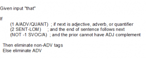
The ENGCG algorithm starts by retrieving all possible tags for each word and then applies the constraints that match, eliminating tags that violate constraints until each word has a unique tag. An example of a constraint is “A past participle cannot immediately follow a pronoun at the start of a sentence.” (This is true because, in the grammar, a past participle requires a preceding auxiliary verb.) A more complex example of a constraint is shown in Figure 4.5. Note that, in the rule shown, “1” means the next word, “2” means the second word to the right of the current word. This rule expresses the constraints associated with selecting the adverbial (ADV) sense of “that” which is a synonym for “very” (as in the sentence “I wasn’t that drunk.” which is a sentence that is not tagged correctly by the default taggers within either NLTK or spaCy, which have been trained on data that likely never saw an example of this construction).
 |
Later versions of the analyzer added information from the XEROX statistical tagger (XT) to remove ambiguities that remained after the applicable rules were applied, eventually reaching an accuracy of over 99.7% compared to the rate of 97% for XT alone. This approach worked better than either using the statistical tagger alone, or using the statistical tagger first. When the errors were reviewed, it was revealed that the hand-written rules tended to solve all but the “hardest” cases of ambiguity, while the statistical model made about 80% of its errors on “easy” cases, but sometimes did better on cases that people think would be “hard”, but were correctly tagged in its training data. (Statistical tagging only got better than rule-based tagging when enough high-quality annotated data was available, e.g., after the competion of the Penn Treebank.)
4.2.2 Brill Tagger
The Brill Tagger, first described in 1993, uses a hybrid of a rule-based and a statistical approach, which can be useful when there is only a limited amount of training data. In this tagger, a simple statistical model is used first and then rules are used to correct specific types of errors observed by experts. Correction rules can be hand-crafted, or learned from an annotated corpus. The algorithm begins by selecting the most frequent category for the word, based on the training data. This is known as a “unigram” model, because it only looks at one word at a time. The rules test for specific suffixes of a word, the surrounding words, and the categories of surrounding words and suggests replacement tags. For example, there is a specific rule for an error in tagging the word “while” in sentences like “She/PRP was/VBD gone/VBN for/IN a/DT while/IN” that occur because “while” is most often a preposition (IN), but in context should be a common noun (NN).
Hybrid tagging addresses the insight that statistical taggers do not always resolve ambiguity correctly, however their errors are generally understandable enough (by experts) to correct by hand using a fixed set of rules. Even when statistical taggers consider more context, and are trained over more data, there will be examples that have not been seen or may not be resolvable without reference to common sense knowledge[8]. A Brill-style tagger, if trained on suitable data, can address the errors seen for a target domain task. A trained instance of Brill’s tagger also requires relatively little space, as it only creates a unigram model. Implementations for versions of the Brill tagger and software for using a corpus to learn rules can be found in the NLTK software library (e.g., nltk.tag.brill and nltk.tag.brill_trainer).
4.2.3 Statistical Classification-Based Tagging
Today, the most accurate POS taggers use sequence classification. The earliest examples used straightforward statistical modelling; more recent ones create models by training neural networks, which allow them to discover novel statistical relationships. The general idea of a sequence-based classifier is to find the ordered list of tags that maximizes the estimated probability of being the correct sequence of tags. This generally involves enumerating and scoring all possible combinations, while keeping track of the best one. Efficiencies can be made by pursuing a greedy strategy that prunes all but the best choice for each word as it moves across a sentence from left to right. Implementations exist that use different statistical models (e.g., Hidden Markov Models, Maximum-Entropy Markov Models, and Conditional Random Fields), which can be implemented by dynamic programming (e.g., the Viterbi algorithm[9]). The newest approaches use various types of neural networks. We will start by discussing the general idea behind sequence classification. Later in Section 4.3.5 we will overview some neural network approaches.
The general idea behind most statistical approaches to language modelling is a two-step process. The first step involves counting the frequency of words and tags within a suitable corpus for subsequences of the original sequence. The second step involves calculating several types of estimated probabilities for each word-tag pair and then selecting the best combination of pairs for the entire sentence. We estimate probabilities when there is no way to get a true probability. The estimates are relatively easy to do by counting. For example, the probability of a single word having a tag can be estimated as the simple proportion of times the word occurs with the tag and to build a bigram model, which is a bit more accurate, we look at words two at a time. To do this we traverse a corpus tagged with part of speech to count and store three things: 1) The number of times that each word occurs with each tag (i.e., C(wi, tj) ); 2) the total number of times that each tag occurs (i.e., C(t)); and 3) the number of times that each pair of tags occurs (i.e., C(ti,ti+1)). Figure 4.6 shows how these counts are used to estimate probabilities, where the real probabilities are on the left, along with the expression used to estimate the value on the right. In line a, we estimate the lexical generation probability because the expression we really want to use (P(t|w)) can be simplified by first using Bayes Rule and then ignoring the P(w) term, since it will be the same for all tags we are considering. In line b, to estimate the probability that tag ti follows tag ti-1, we count the number of occurrences of (ti-1, ti ), divided by the total number of occurrences of ti-1. In line d, we justify combining the estimates for the different parts of the joint probability using simple multiplication by making an assumption that the events can be treated as independent (even though in real life they are not). This is called a Markov Assumption. For real data, where the proportions of counts are very small, we convert the expression in line d to log scale and use addition instead of multiplication to combine the terms. (This conversion is both more efficient and avoids rounding errors.)
| Probability value | Counting-based estimate |
|
a) P(w| t), “the lexical generation probability”
|
C(t,w) ÷ C(t) |
| b) P(ti| ti-1), “the probability a tag follows a given one” | C(ti-1,ti) ÷ C(ti-1) |
| c) P(ti| ti+1), “the probability a tag precedes a given one” | C(ti,ti+1) ÷ C(ti+1) |
| d) P(ti| wi, ti-1, ti+1), probability of a tag for a word |
(C(ti-1,ti)÷C(ti-1)) * (C(ti,ti+1)÷C(ti+1)) * (C(ti,wi)÷C(ti))
– that is, take the product of the three estimates
|
This idea can be extended to longer sequences such as trigrams, or in general ngrams. There is a practical tradeoff between the length of the subsequences used to model a sentence and the number of instances available to train the model. A bigram-based tagger only uses the category of the one immediately preceding word to predict the current one; a trigram-based tagger will use the categories of the two previous words to predict the third. Thus a bigram model will likely include more examples of any given pair. A dataset might have very few of all but the most common triples. When there are insufficient examples of sequences, tagging algorithms can use a backoff strategy, where it applies a sequence of different tagging functions in a fixed order, so that if it does not have enough data to count sequences of length three it will “back off” and use sequences of length two, and so on, or it might default to a rule-based tagger. Another way of avoiding zeros in the calculations for estimated probability is to use a technique called smoothing. Smoothing techniques add very small quantities to the numerator and denominator, just big enough to prevent a zero, without affecting the overall ordering. Examples of smoothing techniques include Laplace smoothing, which adds one to the counts in both the numerator and the denominator and Good-Turing smoothing, which estimates the probability of examples missing in the training corpus by the estimated probability of examples that occur once[10]. One can also build a more complex, and potentially more accurate model, using Conditional Random Fields (CRF). CRFs do not require that one assume independence and also provide a certainty value for different possible sequences. Maximum Entropy Markov Models (MEMM), such as the Stanford CoreNLP tagger, and CRF models do not assume independence so they allow one to use ad hoc features, including suffixes and capitalization, but as a result, they are much slower, and rarely used for relatively simple tasks, such as part-of-speech tagging.
4.2.4 Sequence Classification-Based Tagging with Neural Networks
Statistical taggers are not completely accurate and require a large amount of space to build tables, which can range into the hundreds of millions of entries, in addition to the time they need to compute and compare the estimated probability values. Thus, there has been an interest in alternative methods using neural networks, which compare quite favorably for both accuracy and efficiency, especially for domains which are less standard than newspaper texts, such as micro-blogs[11]. The simplest neural approach uses an Averaged Perceptron, which is a single-layer network (discussed in Chapter 2) that is both accurate and efficient. An implementation of an Averaged Perceptron based tagger became the default tagger for NLTK 3.1 starting in 2017. In that implementation, (originally created by Matthew Hannibal for Textblob[12]), thirteen input features were used, capturing things like the suffixes on the current word and the two preceding words, and the tags on the preceding words (both separately and as a bigram).
The most recent neural network-based implementations use variants of a Deep Learning Architecture, which learn their features rather than depending on experts to select them, making them more adaptable to new domains. This aspect is especially helpful for domains, like microblogs and other types of social media, where nonstandard spelling and out-of-vocabulary words are common. Figure 4.7 shows an example from Twitter and the corresponding tags. (In the figure, UH is the tag for “interjection”, USR is a new tag for “user name”).
| Untagged sequence | @DORSEY33 lol aw i thought u was talkin bout another time . nd i dnt see u either ! |
| Tags as labelled in Gui et al 2017. | USR UH UH PRP VBD PRP VBD VBG IN DT NN . CC PRP VBP VB PRP RB |
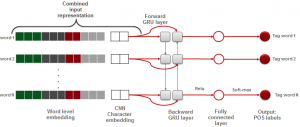
Deep neural network architectures can address nonstandard spellings by using an input representation that maps the word sequence onto vectors or matrices that combine dense word-level representations to capture the general meaning of a word (i.e., a word embedding) with a dense character-level representation of each word (i.e., a character embedding), created using another, previously trained neural network[13]. The number of dimensions for these embeddings can be relatively small (e.g., 32 for the word embeddings and 2 for the character embeddings), compared to the overall size of a vocabulary, which might span hundreds of thousands of words. This combined input structure is then passed to layers that account for sequences (such as a bidirectional Long Short Term Memory layer or a Gate Recurrent Unit layer), followed by some additional layers (e.g., feed-forward or fully-connected) to select the best tags. Figure 4.8 is an illustration of this sort of architecture[14].
 |
An emerging approach that has been proposed for dealing with novel domains is to combine the input with embeddings trained from a domain that is large and more conventional to enrich information from the smaller target domain, an approach known as transfer learning, which has been applied to Twitter text[15]. The tradeoff for these newer models is in the time needed for training. Thus a reasonable approach might start with a pretrained tagger and then address errors with some domain-specific correction rules, if necessary. (One can also provide synthetic training data, meant to teach the model how to handle the erroneous cases.) We will now move to the next stage of syntactic processing which is to identify the syntactic structure over entire sequences of words.
4.2.5 Summary of Part of Speech Tagging
We have just overviewed the four main approaches to word-level tagging: rule-based, hybrid, statistical and heural network based approaches. The task is to which assign to each word a part of speech tag, now generally from the Penn Treebank II tagset, although early approaches, like ENGTWOL used other tagsets. Tagging can be performed separately or included as part of a pipeline.
Now we will consider how structures above the level of an individual word are described and identified computationally.
4.3 Grammars
The assignment of an appropriate syntactic structure to a sequence of words depends on their being some pre-existing notion of what is the correct structure. In NLP syntactic correctness is specified by a grammar. Grammars describe the linear order in which words can occur and, ideally, do so in a way that is generalizable. There are sequences of words that correspond to well-formed constituents and thus longer structures can be specified recursively in terms of these constituents. For NLP work, two general types of grammars are most commonly used, context free grammars (CFG) and dependency grammars. CFGs are used to specify grammars in terms of linguistic categories such as NP and VP are thus are also called “phrase structure grammars” or “constituency grammars”. In a dependency grammar, syntactic structure consists of binary asymmetrical relations (the dependency relations) that hold between words. Information about possible relations is given by the lexical entry for each word, as part of the lexicon that defines the vocabulary of the language. One of the earliest examples was McCord’s Slot Grammar[16]. Figure 4.9 shows the lexical entry associated with the word “given” in a McCord’s lexicon. The entry says that given is a past participle and has three relations: subject (subj), direct object (obj), and indirect object (iobj). Formally, a lexical entry can also be given as a combination of the word and a pair of finite state automata that define what relations exist to the right and to the left of the word, respectively [17].
|
Parsing is the computational process of determining the correct structure for a given sequence of words, given the specification provided by the grammar. Parsing can use search or classification. A search-based parser traverses either the words of the sentence or the rules of the grammar to find a match between subsequences of the words and the rules of a grammar. Grammars for language tend to overgeneralize, resulting in thousands of possible parses, so the best approaches rely on mechanisms for ranking and pruning, so that only the most likely structures are considered. Like machine learning-based approaches, the algorithms for determining the most likely structures make use of information from a dataset of previously parsed sentences to estimate probabilities.
A classification-based parser takes a model that has been learned from sentences previously annotated with the correct parse in the target format and applies it to an unparsed sentence to determine which of its previously seen structures (or equivalently, previously seen sequences of parser actions) is best according to that model. The coverage and accuracy of a classification-based parser thus depends on a combination of the quality of the training set and the sensitivity and specificity of the modelling algorithm.
4.3.1 Context Free Grammars
Context Free Grammars (CFGs) are a formalism for describing both the syntactic structure of human language and of programming languages. The formalism was developed in the 1950’s and applied to describe natural language syntax by Noam Chomsky[18]. A CFG consists of a set of re-write rules, A -> B1 B2 … Bn, where symbols that appear on the left-hand side (LHS) are called “nonterminals” and the symbols on the right-hand side (RHS) can be either nonterminals or terminals. The terminal symbols are those that do not appear on the left-hand side of any rule, because they are “atomic” for the language in question. In a grammar for a human language the terminals are the words and the nonterminals are phrase categories such as NP, VP, and S. Every CFG also has a distinguished “root” nonterminal that can serve as a starting place for a top-down search or an ending place for a bottom-up search. CFGs can have any number of symbols on the RHS, but the most efficient algorithms for parsing CFGs require that the rules all be binary (i.e., have exactly two symbols on the RHS. A nonterminal can have more than one RHS, in which case they are defined as separate rules, although parsers also allow an abbreviated notation, where the different RHS are listed together, separated by a vertical bar.
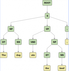
Parse trees are a way of depicting the derivation of a sequence according to the grammar. In trees, the root nodes are the nonterminals of the grammar, the leaf nodes are the words. Figure 4.10 shows an example of a parse tree for a phrase structure analysis of the sentence “The dog ate the beef”.
 |
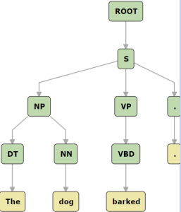
A CFG can be defined explicitly, after a qualitative analysis of a language (such as described in Chapter 3), or it can be induced from a dataset where sentences have been previously annotated with their correct parse, i.e., a treebank. To induce a grammar, a computer algorithm can traverse all the trees starting from the root and for each subtree that has children, create a rule where the root of the subtree is the LHS nonterminal and its children form the RHS. Figure 4.11 shows the rules that might be learned from a parse of the sentence “The dog barked.” If the parse trees in the data set had more than two branches, but a binary branching grammar is desired, then the induced rules can be rewritten using additional nonterminals to create binary trees. For example, the rule NP-> DT NN CC NN PP, can be rewritten as NP -> DT N1 and N1-> N1 PP | N1 CC N1, where N1 is a new nonterminal. Terminals are just the words, which can be collected directly from the unannotated text or from the treebank.
| Parse tree | Induced rules |
 |
|
4.3.2 Probabilistic Context Free Grammars
Probabilistic Context Free Grammars (PCFG) are a variant of context free grammars where each rule is annotated with a numerical value that expresses the likelihood that the rule will be used when rewriting the terminal on the left-hand side. The numbers follow the conventions of a probabilities where the sum of the values for the same nonterminal must equal 1. Figure 4.12 shows an example of a small PCFG.
| Grammar | Probability | Lexicon | Probability |
| S → NP VP | 1.0 | NN → talk | 0.6 |
| NP → DT NN | .4 | NN → money | 0.4 |
| NP → NN | .2 | NNS → talks | 1.0 |
| NP → PRP$ NN | .3 | PRP$ → my | 0.4 |
| NP → PRP$ NN NNS | .1 | PRP$ → your | 0.6 |
| VP → VBZ | .6 | RB → loudly | 1.0 |
| VP → VBZ RB | .4 | VBZ → talks | 1.0 |
PCFGs can be created by hand, as in Figure 4.12 but in practice they are usually induced from annotated collections of bracketed sentences or a treebank. Bracketed sentences (also called shallow parses) include only the top-level phrase categories, and are used when full trees are not available or needed. Figure 4.13 shows some sample bracketed data that might be used to induce a PCFG.
| Pattern Type | Count |
| [S [NP] [VP]] | 300 |
| [S [VB] [NP]] | 100 |
| [S [S [NP] [VP]] [CC] [S [NP][VP]]] | 200 |
For the example in Figure 4.13, we must also consider the phrase types within a pattern. So in Figure 4.13 there are 700 examples of “S →NP VP“ (including 400 that appear nested within the third type of pattern). There are 100 examples of “S → VB NP” and 200 examples of “S → S CC S“, resulting in a probability of assignment for the PCFG sentence rule of S → NP VP [0.7] | VB NP [0.1] | S CC S [0.2].
Simple PCFGs provide a way to resolve local syntactic ambiguity, but they are not always very accurate, because many ambiguities depend on relationships between specific words, as in “They ate udon with forks.” versus “They ate udon with chicken.” Often accuracy can be improved by conditioning the probabilities by the word that is the head of the constituent (such as the main verb in a verb phrase or the main noun in a noun phrase). Figure 4.13 gives an example rule by Collins[19] that might be used for finding the head of a noun phrase.
|
If the rule contains NN, NNS, or NNP: Else If the rule contains an NP: Else If the rule contains a JJ: Else If the rule contains a CD: Else Choose the rightmost child |
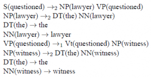
Collins used rules like this to define a lexicalized context free grammar (LCFG), which includes the head words for each phrase. Figure 4.14 shows an example of a lexicalized CFG (shown without estimated probabilities).
 |
Another way to improve PCFG grammars is to combine the syntactic categories of a PCFG with a neural network that learns vector representations that combine syntactic and semantic information. This approach, called a Compositional Vector Grammar (CVG)[20], uses a neural network to learn weights for each nonterminal. The CVG captures the notion of head words that are needed for ambiguities that require semantic information, such as PP attachments, and also addresses the problem of sparsity, because it generalizes over similar words (e.g., words that had similar neighbors) in the training data.
4.3.3 Dependency Grammars
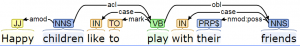
Dependencies are asymmetric binary relations that express the functional role of the word with respect to another word that is considered the head of the relation. These relations form head-dependent pairs. Researchers have refined and standardized the types of dependency relations, following the work on creating lexicalized context free grammar rules. There are three general types of relations: relations that specify modifiers, relations that specify complements (required arguments), and relations which essentially name the type of word itself, such as determiners, conjuncts, and copula. The most standardized set of dependency relations and their definitions is maintained by the Universal Dependency organization. Figure 4.15 shows an example dependency tree, which groups all the dependencies originating at the same word together at a single node. Note that unlike a constituency tree, the words are root nodes and the dependencies are labels on the edges between them.
The specifications of dependency grammars can be specified by hand, in the lexicon, as in the original slot grammars described above, or they may be induced from treebanks. It has been shown that dependency grammars and context free grammars are equivalent in expressiveness, and dependency grammars can be learned from either treebanks based on constituency (such as the Penn Treebank) or tree banks created using dependency parsers. Using a treebank, dependency grammars and parsers can be augmented with estimated probabilities (in a manner similar to PCFGs), including creating rules that are conditioned on the specific head-dependent pairs.
In the next sections, we will consider parsing algorithms for both constituency and dependency grammars, considering both search and classification-based approaches to parsing.
4.4 Search-Based Parsing
The most widely used search-based algorithms for parsing are the CKY algorithm (named for its creators: Cocke, Kasami, and Yonger), and the Shift-Reduce Algorithm. Both CKY and Shift-Reduce are “bottom-up” algorithms, which means they begin the parse with individual words, and work their way “up” towards a structure that spans the entire sentence. (Bottom up algorithms are also useful for traversing a parse tree, for example to compute a semantic representation in a compositional way.) CKY is relatively efficient (for a bottom up algorithm), because it can be implemented as dynamic programming using a matrix to keep track of partial results. An example of a CKY algorithm, is bottom-up chart parsing, which can also make use of rules annotated with probabilities or semantics. It is also used in some neural neural network approaches to build the final result.
Because bottom-up chart parsing has so many applications, we will be doing an in-depth dive into the algorithm.
4.4.1 Chart Parsing
Chart parsers create structures, called edges, to represent both complete constituents and partially complete constituents (of a sentence). The partially complete structures allow them to make predictions about what will be processed next and to use those predictions to guide the parse. Each edge stores the grammar rule that is being used and locations where it begins and ends. By convention, locations begin at 0 (zero) just before the first word, and end just after the last word of the constituent. Figure 4.16 is an example of a sentence, marked with locations, showing all possible spans for the sentence “The cat ate a mouse”, listing all spans of length 1, all of length 2, etc. We use the notation [i:j] to describe the span of words from location i to location j and [k:k] to describe the point just before processing the word that begins at location k. For example, in Figure 4.16, [0:2] corresponds to “the cat” and [2:2] is the location before “ate”. Chart parsers can be used both for parsing context free grammars, and for dependency parsing. For clarity, we will consider chart parsing only using a simple CFG. (We will consider parsing with dependencies when we discuss transition-based dependency parsing in the next section.)
| 0 | 1 | 2 | 3 | 4 | 5 | |
| Spans of length 1 | The | cat | ate | a | mouse | |
| Spans of length 2 | The | cat | a | mouse | ||
| Spans of length 3 | ate | a | mouse | |||
| Spans of length 5 | The | cat | ate | a | mouse |
Chart parsing is an exhaustive enumeration of all edges induced by a grammar—any and all grammar rules that can match will result in an edge being added to the chart. The more ambiguity a grammar allows, the more edges will be created. Figure 4.17 shows the edges we would get if we used a context free grammar along with all the parts of speech for each word as found in a typical dictionary, using the tags of the Penn Treebank tagset (e.g., JJ is “adjective” and RB is “adverb”). Here, the word “the” has two parts of speech (DT, IN, RB), “horse” has four (NN, JJ, VB, and VBP), “raced” has two (VBD, VBN), “past” has four (NN, IN, JJ, and RB), “barn” has one, and “fell” has three (NN, JJ, VBD)[21]. To the left, the figure shows all the edges of length 1 that could be created by matching rules from the bottom up.
|
Sentence: |
||||||||||||||||||||
|
The edges that are created to keep track of the state of a parse before a rule is completely matched are called “active edges”. As the sentence is processed from left to right, for each partially matched grammar rule, the algorithm will create an active edge to store what has been matched, and what is still needed. A dot (*) is used to designate the dividing point between what has been matched and what is still needed. (If an edge is created with no parts matched, then the dot will be immediately after the arrow, as in A → * B1 B2.) As more parts are matched, new edges are added, with the dot moved over to the right. When the dot reaches the far right end of a rule, then the edge is “complete” (also called “inactive”) and it can be used to extend other active rules. Figure 4.18 shows another small grammar and some edges that would be created, midway through the parse.
|
Sentence:
|
||||||||||||
|
The steps in a bottom up chart parsing algorithm can be specified by the two parsing rules shown in Figure 4.19. These rules describe how to combine edges to create longer edges.
Bottom-up rule: When a new category is seen (or nonterminal rule for that category is completed completed), then for any rule where that category is leftmost on the RHS, create a new edge with the dot just to the left of the category. If ( ([i:j], X) or [i:j] X -> U V *) and A -> X Y, then add ([i:i], A -> * X Y) Note: Y can be empty.
Fundamental rule: When a new category is seen or nonterminal created, then for all active rules where the category is leftmost on the RHS of the dot, and the spans are adjacent, create a new edge with the dot moved to the right of that category and combine the spans. If ([i:j], A -> X * Y Z and [j:k] Y -> U V *, then add ([i:k], A -> X Y * Z) Note: X and Z can be empty. |
In practice, CKY can be most efficiently implemented as dynamic programming using a two dimensional matrix. In dynamic programming, instead of explicitly representing a location [i:j] when we parse a sentence of length N, we create an N by N matrix and store the edges with span [i:j] at row i and column j in the matrix[22]. Then, for any complete parse with topmost rule S → X Y, there would be an edge ([0:N], S → X Y *). Figure 4.20 shows the pseudocode for the CKY algorithm as dynamic programming. To start, we place the words or unary lexical rules at their corresponding locations. then we iterate over all possible lengths of spans, starting at 2 and ending at the length of the sentence, and for each span length we iterate over all locations in the table. Then we iterate over all possible edges, from all possible starting points, and apply bottom up and fundamental rules wherever they would apply. (The pseudocode does not list the empty edges created by the bottom up prediction rule, but they are shown in the trace shown in Figure 4.21 that follows.)
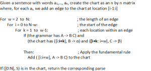 |
Figure 4.21 shows a bottom up chart parse of the sentence “The dog barked.”, along with the corresponding active and inactive edges and their placement within a matrix when using dynamic programming. This trace follows the implementation of the bottom up chart parsing algorithm as implemented in NLTK. (It also follows the convention that when matrices for a chart parse are shown, they are shown with the vertical axis reversed so that the parse appears in the upper right corner.)
| Matrix values | Edges in chart | Parser actions |
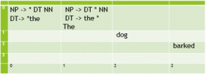 |
[0:0] DT → *the [0:1] DT → the * [0:0] NP → * DT NN [0:1] NP → DT * NN |
Predict the, and apply the fundamental rule to create a completed edge from 0 to 1. Predict bottom up an empty NP (* NP) and apply the fundamental rule to get NP -> DT * NN. |
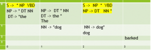 |
[0:0] DT → *the [0:1] DT → the * [0:0] NP → * DT NN [0:1] NP → DT * NN [1:1] NN → *dog [1:2] NN → dog * [0:2] NP → DT NN * [0:0] S → * NP VBD [0:2] S → NP * VBD |
Predict dog and apply the fundamental rule to create a completed edge from 1 to 2. Apply fundamental rule to complete the NP at [0:2] and extend the S, to get S -> NP * VBD. |
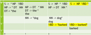 |
[0:0] DT → * the [0:1] DT → the * [0:0] NP → * DT NN [0:1] NP → DT * NN [1:1] NN → * dog [1:2] NN → dog * [0:2] NP → DT NN * [0:0] S → * NP VBD [0:2] S → NP * VBD [2:2] VBD→* barked [2:3] VBD→ barked * [0:3] S → NP VBD * |
Predict barked and apply the fundamental rule to complete VBD and apply the fundamental rule again to complete the S. |
In practice, when using a bottom-up chart parsing algorithm, there will be huge number of possible edges and so some mechanism is needed to prune edges that are not likely to be part of the final parse. This difficulty is the primary reason for using a probabilistic context free grammar (PCFG). When using a PCFG rather than a CFG, the CKY algorithm is adapted to use the probabilities values associated with each rule in the grammar. For simplicity, the probabilities are treated as independent, which means that during parsing they are combined using multiplication. The probability of a parse tree will be calculated as the product of the probability of the rule for the root times the product of the probabilities associated with each of the subtrees (i.e.,, categories on the right-hand side). Thus, for the grammar shown in Figure 4.12, the probability for the sequence “Your money talks” as a NP would be calculated as the product “0.1*0.6*0.4*1.0” (0.024), whereas the probability for a S would be the product “1.0*0.3*0.6*0.4*0.6*1.0” (0.0432). When multiple parses for a span [j:k] of text are possible, the CKY algorithm for PCFG will store, for each nonterminal X at location [i:j], the highest probability parses found for X, a variant of beam search, where the beam can be 1, 1000, 10000, or whatever seems suitable. When a PCFG is lexicalized, the process is similar, except that when the product for the entire parse tree is computed, there is an additional multiplicand for the estimated probability (based on the frequency in the source corpus) associated with the top level S having the designated lexical head (e.g., S(talks)); so if “talks” occurs as the main verb for 2 sentences out of 1000, for the sentence above, we would multiply 0.002 with the 0.0432).
4.4.2 Shift-Reduce Parsing
A Shift-Reduce parser, also called a transition-based parser, maintains the state of the current parse and applies transitions that update the parse state, such as combining two inputs or combining an input with a previously built structure. When implemented as a search procedure, the state is usually represented using two data structures: a queue of words to be parsed and a stack of partially completed structures. (In some cases, the parser also maintains an agenda of the best partial parse states.) The initial state has all the words in order on the queue and an empty stack. At each parsing step, the parser selects and applies transitions to the current state until its queue of inputs is empty and the current stack only contains a finished tree.
The two main types of transitions are shift, which is where a word moves from the queue onto the stack and reduce, which is where nodes on the stack are combined and relabeled. Implemented SR parsers may use additional transitions (such as “accept”, “finalize,” or “idle”) or specialize the reduce action into several subtypes (e.g., based on the lexical head), to control the parsing process or make it more efficient. Shift-reduce parsing can either be used to do constituency parsing for context free grammars or dependency parsing. It has also been used in the implementation of compilers for programming languages. Figure 4.22 below gives an example of a small CFG grammar and a sample parse, for the expression “T and T”, where “$” is used to indicate the bottom of a stack or the back of a queue.
| Sample grammar | Sample parse | ||||||||||||||||||||||||||||||||||||||||
|
|
For constituency parsing, with a grammar rule A → B C, a reduce operation might replace two nonterminals B and C by the LHS nonterminal A. For a dependency grammar, if the top two items on the stack could be linked by a dependency relation, the items will be removed and replaced by the one that is considered the head, such as the verb in an nmod relation, and the relation added to another data structure. We will consider another example of shift reduce parsing in the next section, when we discuss Dependency Parsing.
As with probabilistic context free parsing, shift-reduce parsing may be adapted to use a scoring function to choose what type of transition to apply in each state when there are multiple options. These scoring functions are normally learned from data, either as probabilities estimated from a treebank or as values derived from trained neural network models. A shift-reduce parser might be greedy about transitions, always choosing the option that scores best. Or, it might implement a type of beam search (see Chapter 2) where only the a subset of top-scoring partial states are kept on the agenda and continues until the highest scoring state on the agenda is finalized. Beam search can provide better accuracy in less time, but it requires models that were specifically trained to work with beam search. A model not trained for beam search only has features for states reached for the correct parse trees. By contrast, a model trained to use beam search also trains with negative features for incorrect states on the beam, (i.e., features for phrase-level ambiguities that were not part of the final parse) resulting in many more features and therefore a much larger model.
4.4.3 Search-Based Dependency Parsing
First we will consider how dependency parsing can be understood using search; in the next section we will reconsider dependency parsing as classification-based parsing. Dependency parsing involves choosing for each word, what other word it is related to as a dependent. By convention, the top-level node is called the root and the main verb is its dependent. A variety of search-based algorithms have been used to build dependency structures including ones based on: dynamic programming, maximum spanning trees, constraint satisfaction, or greedy algorithms, similar to those already discussed, although some also combine supervised machine learning to get better results[23].
Search-based dependency parsing algorithms all start the search with the main verb and then try to generate dependents by traversing the different types of edges known to be associated with the root, based on subcategorization information (see Chapter 3) stored in the lexicon. For example, in the sentence: “I baked a cake in the oven.” the main verb (root) is “baked”. The verb has a noun subject (nsubj) relation to “I”. There is a determiner (det) relation between “cake” and “a”. There is a determiner object (dobj) between “cake” and “baked” . There is a case relation between “oven” and “in” and a determiner (det) relation between “oven” and “the”. There is a noun modifier (nmod) relation between “cake” and “oven”.
Naive dependency parsing algorithms based on breadth first search consider and score all possible combinations of head and dependent – which leads to a Big-O complexity of O(n5), but McDonald et al’s (2005) approach is O(n2). Using a corpus annotated with dependency trees, a classifier is trained to compute a score for each type of edge. The types of features include: the head word, the dependent word, and part of speech (POS), separately; the head word, dependent word and POS, as bigrams (e.g., (the, DT)); the words between head and dependent; and the length and direction of the dependency. The training is based on maximizing the accuracy of the overall tree. The classifier is then used to discriminate among alternative trees, where the score of a tree is calculated as the sum of the score of the dependencies. An alternative classifier-based approach involves training classifiers to optimize the actions of a shift-reduce parser[24],[25]. The algorithms extend the traditional operators of a shift-reduce parser to include different types of reduce operators for the different types of edges and directions of the edges, to allow for more accurate scoring. Once actions are scored, then a greedy search algorithm can be used to select the actions that comprise the single best parse or a beam search can be used to select from just a subset of the best scoring ones.
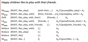
Figure 4.23 shows the start of a shift-reduce dependency parse of the sentence “Happy children like to play with their friends.” In the figures, the first column shows the action (where LA and RA designate two types of attachment, left and right respectively). LA attaches the front element of the queue to the top of the stack with the element taken from the queue placed on the left; RA attaches the front element of the queue to the top of the stack with the element on the right. The subscript shows the type of dependency, such as amod. The second column shows the symbols that have been shifted from the input buffer onto the stack. The third column shows the queue remaining input; and the last column shows the set of dependency structures that have been created.
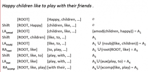 |
Figure 4.24 shows the last few steps of the same parse. Note, if one were to draw a tree at the same time, every shift action would create a sibling whereas each LA/RA adds a new edge between a head and a dependent. In Figure 4.24, the “Reduce” actions at the end of the parse remove items from the stack without creating any new dependencies. The parse ends when the queue (column 3) is empty.[26].
 |
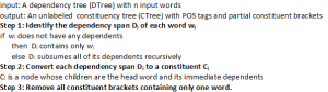
Shift-reduce dependency parsers can use information learned from a corpus to score the actions of a shift-reduce parser to resolve ambiguities, similar to the scoring method used to rank alternatives with a PCFG, by selecting actions that result in more commonly seen structures. The treebanks for training dependency parsers can either be ones that include dependency trees, or they can be adapted from phrase structures, as found in the Penn Treebank. There are also algorithms for translating dependency trees into phrase structures[27], [28]. In the more recent work of Lee and Wang[29] dependency structures are mapped to constituent trees in a two-phase process, as shown in Figure 4.25, where the first phase traverses the dependency structure to construct a partial set of constituent spans and the second phase applies a constraint-based maximum entropy parser[30], a type of statistical parser similar to a shift-reduce parser, to the original sentence to select the best phrase-level nodes.
 |
4.5 Classification-Based Parsing
Most large-scale parsers developed since 2015 use sequence classification as the primary method rather than search. Most are also targeted to producing a dependency structure, because the structures are more language independent and sufficient for many downstream tasks. However, neural constituency parsers also exist. Versions exist that provide either a single best parse or a few best alternatives via a beam search. The training for a beam search is different than for a single-best parser. A single-best model only uses features or states that were associated with the correct parse found in the training set. A model that can return and rank multiple alternatives must also train negative features to prevent poorer quality alternatives from becoming part of the final set. Most approaches to supervised machine learning have been applied to model language at the sentence level, including linear models (such as Support Vector Machines), shallow neural networks (such as Perceptrons), and deep networks, which are fast emerging as the dominant approach [31].
4.5.1 Classification-Based Constituency Parsing
Modern classification-based constituency parsing uses deep neural networks. These networks do not require a grammar or lexicon, all knowledge is embedded in the language model that has been learned by processing a training dataset that includes parse trees. For a constituency parser, these parse trees must be constituency trees, such as found in the Penn Treebank. Current approaches often use an internal data representation similar to chart, consisting of labelled spans, e.g., (0, 2, NP) . For an internal representation based on charts, there are three aspects: representations of tokenized input, representations of spans, and scoring mechanisms for labels. The input layer comprises representations for several types of information for each word: word meaning, word position in the sentence, and part of speech, usually as embeddings that are learned as part of the overall training with the treebank, but they can be learned separately and input pretrained. The internal layers are often a bidirectional Long Short Term Memory (LSTM), which is one that operates on both a forward and a reversed version of the sentence[32], or a self-attentive encoder[33], to account for constraints from either side of the sentence surrounding the word. (In a self-attention model, nodes can focus on locations, and the weight of each is also a learned value, independent of the number of intervening words, to account for long-distance interactions, such as for questions where the wh-word seems to have been moved to the front.) These layers generate a score for each combination of a label and a span. The final stage of constituency parsing networks is typically a decoder to generate trees, by performing a CKY-style bottom up traversal that builds a tree comprising the highest-scoring labelled spans.
4.5.2 Classification-Based Dependency Parsing
Classification based approaches to dependency parsing also now use deep neural networks, trained using a dependency treebank. These networks are trained to jointly select: a) pairs of words that are optimally head and dependent and b) optimal dependency relations for candidate pairs (head and dependent words). In the final layer, the scores of all candidates are examined to select the best one. When training the network, the overall loss to be minimized is a combination of the loss (e.g., a sum) for the component subproblems. In intuitive terms, these networks are trained to provide a score that is akin to an estimated joint probability of the head, dependent, and relation, based on the “context” of the sentence. However, scores may not be limited to values between 0 and 1 and, for these networks, context is not a simple matter of nearby word or part of speech tag, but instead includes vector representations for a wide range of features such as part of speech tags, morphological features, character sequences, word types (as both a lemma and a semantic embedding), and sometimes scalar values to indicate the linear order and the distance between the head and the argument. These input vectors allow the networks to generalize over minor variations in spelling, meaning, or syntactic expression.
One of the most accurate (and most complex) exemplars of the neural classification approach has been developed by the Stanford NLP group. Their current implemented NLP pipeline is called Stanza and an illustration of the overall architecture is shown in Figure 4.26[34]. Designed to allow input as raw text, the pipeline of Stanza uses a complex neural architecture involving several layers to first create separate embeddings for each type of information (e.g., multiple layers of biLSTM, a final LSTM layer, several layers of Rectified Linear Units (ReLU), followed by additional layers to perform matrix operations that combine the separate vectors to select the optimal head, dependent, and relation combinations[35], [36]. Most of the processes listed on the left have been discussed previously, except “multi-word token expansion” which would handle things like mapping contractions onto separate tokens (e.g., “don’t” onto “do and not”) and named entity recognition, which is a type of shallow semantic processing that labels proper nouns and expressions with their general type, such as person, organization, location, etc. (We will discuss named entity recognition in a later chapter.)
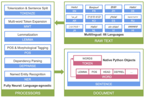 |
Stanza has has been implemented in Python, using the PyTorch software libraries for machine learning. It is open source, but may not be suitable for everyone, as it runs best on a GPU-enabled machine. Simpler architectures, using fewer layers, also do quite well, including UDPipe, which achieves 70 to 85% accuracy, runs on common laptops, and has libraries implemented for several programming languates[37], [38].
Classification-based parsers are available as parts of nearly all recent NLP software libraries. These libraries include one or more pretrained models for large widely used datasets, but also provide instructions and tools for updating or training models with new data. Data for training neural networks for dependency parsing must usually be provided in what is known as the CoNLL-U format, which is an ASCII format defined for a series of yearly task-based challenges (which are conferences with a common data set where participants submit results for prespecified tasks using the data)[39].
4.6 Shallow Parsing
Some applications do not require a full parse of the sentence, just a subdivision of the text into the top-level phrases. This process is called shallow parsing or chunking, Shallow parsing can involve either the creation of regular expressions to identify boundaries or the training of a classifier to find the end points of chunks.
4.6.1 Regular Expressions for Chunking
The grammars used for chunking are defined as complex regular expressions, which are similar to context free grammars, but typically do not involve recursion. For example to say that an NP chunk should be formed by a sequence of an optional determiner (DT) followed by any number of adjectives (JJ) and then a noun (NN) or as a sequence of proper nouns, one would use the regular expression “NP: {<DT>?<JJ>*<NN>}{<NNP>+}” in NLTK, where “?” indicates optional, “*” means occurs “zero or more” times, and “+” means “one or more” times.
When regular expression parser runs, it searches for sequences of tokens that match the pattern and produces a list, with each matched sequence labelled with the pattern type. To be able to define and use patterns recursively, one typically must iterate over the grammar multiple times, corresponding to the maximum depth of recursion that is allowed. Figure 4.27 shows an example, adapted from Figure 7.10 of Chapter 7 of the NLTK book[40], that illustrates the use of a recursive (cascaded) chunk grammar. NLTK does allow some recursion with regular expression-based chunking, but only if given a maximum depth, as done with the “loop=2” parameter in this example. By contrast, a CKY or Shift-Reduce parser will perform recursion to an arbitrary depth.
| RegEx grammar |
|
| Chunk grammar |
|
4.6.2 Classification-Based Chunking
To annotate chunks for training a classifier, some systems use an encoding that is called CoNLL 2000, because it is based on the encoding used from that conference. That encoding combines POS tags with labels that indicate the beginning (B) and inside (I) of the chunks, and use O tags to indicate “outside a chunk”. An extended version of this encoding (CoNLL 2002) combines POS tags with semantic types for named entities, which are proper name expressions such as for people, organizations, or locations. Figure 4.28 shows examples of these two encodings with chunks on the left and named entities on the right. With training data labelled with CoNLL tags, a sequence classifier can be used to learn to tag unseen data, and expressions extracted by merging adjacent sequences of tokens that have related tags, e.g., [B-Loc, I-Loc, I-Loc], terminated by an “O” tag. Other similar encoding strategies are sometimes used.
|
Encoding of Chunks |
Encoding of Named Entities |
|
|
As a start, one might also try using a prettrained NER tagger, such as found in a software toolkit such as spaCy or CoreNLP. The taggers can be invoked by running the complete pipeline (the usual case), or one can call a tagger separately, after first splitting the text into separate words using “split()”[41].
4.7 Summary
This chapter considered tasks associated with identifying the syntactic structure of natural language including tokenization, part-of-speech tagging, grammars, and parsing. We considered two types of analyses: parsing to identify syntactic constituents, such as phrases and clauses, and parsing to identify dependency structures, the sets of binary relations that connect the head words of constituents. Grammars describe what sequences comprise a language. Identifying how words or sequences match the grammar can be done by either a search process or classification. Creating datasets for classification is typically accomplished in a semi-automated manner: first, apply a search-based parser and then hand correct the analyses. Pretrained language models can sometimes be extended without adding new data, by enhancing the input representations to include semantic information (using word embeddings) or to include character-level embeddings where dense vectors are trained to map strings of characters (including those for non-standard spellings) onto known words. Although dependency structures provide information about syntactic function, it should be noted that this is not the same as a meaning representation or semantics. In the next chapter we will consider what sorts of semantic representations are possible and computational methods for creating them.
- Universal Dependencies.org (2021) The English Web Treebank URL: https://universaldependencies.org/treebanks/en_ewt/index.html ↵
- Devlin, J., Chang, M., Lee, K., and Toutanova, K. (2019). BERT: Pre-training of Deep Bidirectional Transformers for Language Understanding. NAACL-HLT. ↵
- Google Research (2019) Github site for bert tokenizer URL: https://github.com/google-research/bert/blob/master/tokenization.py ↵
- A mapping from PTB tags to UD tags can be found online at: https://universaldependencies.org/tagset-conversion/en-penn-uposf.html ↵
- Marshall, I. (1983). Choice of Grammatical Word-Class without Global Syntactic Analysis: Tagging Words in the LOB Corpus. Computers and the Humanities, pp.139-150. ↵
- One can download the GENIA tree bank from https://nlp.stanford.edu/~mcclosky/biomedical.html CMU distributes POS taggers trained for either Twitter Data or data from the English Web Treebank; you can find it at http://www.cs.cmu.edu/~ark/TweetNLP/#pos ↵
- Samuelsson, C. and Voutilainen, A. (1997). Comparing a Linguistic and a Stochastic Tagger. In Proceedings of the 35th Annual Meeting of the Association for Computational Linguistics and Eighth Conference of the European Chapter of the Association for Computational Linguistics Association for Computational Linguistics (pp. 246-253). ↵
- Young, S. and Bloothooft, G. eds. (2013). Corpus-based methods in Language and Speech Processing (Vol. 2). Springer Science & Business Media. ↵
- Forney, G.D. (1973). The Viterbi Algorithm. In Proceedings of the IEEE, 61(3), doi: 10.1109/PROC.1973.9030, pp.268-278. ↵
- Zhai, C. and Lafferty, J. (2004). A Study of Smoothing Methods for Language Models Applied to Information Retrieval. ACM Transactions on Information Systems (TOIS), 22(2), pp.179-214. ↵
- Banga, R., and Mehndiratta, P. (2017). Tagging Efficiency Analysis on Part of Speech Taggers. (2017). International Conference on Information Technology (ICIT), Bhubaneswar, doi: 10.1109/ICIT.2017.57. pp. 264-267. ↵
- Loria, S. (2020). Textblob: Simplified Text Processing, URL: https://textblob.readthedocs.io/en/dev/ ↵
- Pytorch.org 2017. Sequence Models and Long-Short Term Memory Networks URL: https://pytorch.org/tutorials/beginner/nlp/sequence_models_tutorial.html ↵
- Meftah, S. and Semmar, N., (2018). A Neural Network Model for Part-of-Speech Tagging of Social Media Texts. In Proceedings of the Eleventh International Conference on Language Resources and Evaluation (LREC 2018). ↵
- Gui, T., Zhang, Q., Huang, H., Peng, M., and Huang, X.J. (2017). Part-of-Speech Tagging for Twitter with Adversarial Neural Networks. In Proceedings of the 2017 Conference on Empirical Methods in Natural Language Processing (pp. 2411-2420). ↵
- McCord, M.C. (1990). Slot Grammar. In Natural Language and Logic (pp. 118-145). Springer, Berlin, Heidelberg. ↵
- Alshawi, H. (1996). Head Automata and Bilingual Tiling: Translation with Minimal Representations. In Proceedings of the 34th Annual Meeting on Association for Computational Linguistics (pp. 167-176). Association for Computational Linguistics. ↵
- N. Chomsky, (1956) "Three Models for the Description of Language," in IRE Transactions on Information Theory, 2(3):113-124. doi: 10.1109/TIT.1956.1056813. ↵
- Collins, M. (1999). Head-Driven Statistical Models for Natural Language Parsing. Ph.D. thesis, University of Pennsylvania ↵
- Socher, R., Bauer, J., Manning, C.D. and Ng, A.Y. (2013). Parsing with Compositional Vector Grammars. In Proceedings of the 51st Annual Meeting of the Association for Computational Linguistics (Volume 1: Long Papers) (pp. 455-465). ↵
- Occurrences of some of some of these parts of speech are very rare and thus may not be familiar. For example, "horse" can be tagged as a noun (NN) as in "I saw a horse.", or an adjective (JJ) as in "I visited a horse farm." or a base form of verb (VB) as in "I wanted to horse around." or a present tense verb (VBP) as in "I horse around with my kids". ↵
- CKY assumes that all rules in the grammar (except lexical rules) have exactly two nonterminals on the right hand side - or has been binarized by adding extra nonterminal symbols. ↵
- McDonald, R., Pereira, F., Ribarov, K. and Hajič, J. (2005). Non-Projective Dependency Parsing using Spanning Tree Algorithms. In Proceedings of the 2005 Conference on Human Language Technology and Empirical Methods in Natural Language Processing (pp. 523-530). Association for Computational Linguistics. ↵
- Yamada, H. and Matsumoto, Y. (2003). Statistical Dependency Analysis with Support Vector Machines. In Proceedings of the Eighth International Conference on Parsing Technologies (pp. 195-206). ↵
- Nivre, J. (2008). Algorithms for Deterministic Incremental Dependency Parsing. Computational Linguistics,34(4), pp.513-553. ↵
- Note, this example traces a correct parse of "Happy children like to play with their friends." The Stanford CoreNLP.run online demo did not produce this parse when this example was written. It gave the following wrong one instead:
 The most recent Stanford parser may address this, however. ↵
 - Collins, M., Ramshaw, L., Hajič, J. and Tillmann, C., (1999). A Statistical Parser for Czech. In Proceedings of the 37th Annual Meeting of the Association for Computational Linguistics (pp. 505-512). ↵
- Xia, F. and Palmer, M. (2001). Converting Dependency Structures to Phrase Structures. In Proceedings of the First International Conference on Human language Technology Research (pp. 1-5). Association for Computational Linguistics. ↵
- Lee, Y. S., and Wang, Z. (2016). Language Independent Dependency to Constituent Tree conversion. In Proceedings of COLING 2016, the 26th International Conference on Computational Linguistics: Technical Papers (pp. 421-428). ↵
- Adwait Ratnaparkhi. 1997. A Linear Observed Time Statistical Parser Based on Maximum Entropy Models. In Proceedings of Empirical Methods in Natural Language Processing (EMNLP). Also in ArXiv.org URL: https://arxiv.org/abs/cmp-lg/9706014 ↵
- See Linzen, T. and Baroni, M. (2020). Syntactic Structure from Deep Learning. arXiv preprint arXiv:2004.10827. URL:https://arxiv.org/pdf/2004.10827 ↵
- Gaddy, D., Stern, M. and Klein, D., 2018. What’s Going on in Neural Constituency Parsers. An Analysis. In the Proceedings of the 16th Annual Conference of the North American Chapter of the Association for Computational Linguistics: Human Language Technologies. Also online as: https://arxiv.org/pdf/1804.07853.pdf ↵
- Kitaev, N. and Klein, D. (2018). Constituency Parsing with a Self-Attentive Encoder. arXiv preprint arXiv:1805.01052. ↵
- Qi, P., Zhang, Y., Zhang, Y., Bolton, J. and Manning, C. (2020). Stanza: A Python Natural Language Processing Toolkit for Many Human Languages. In the Proceedings of the 58th Annual Meeting of the Association for Computational Linguistics (ACL) System Demonstrations. Also see the STANZA Github website: https://stanfordnlp.github.io/stanza/ ↵
- Dozat, T., Qi, P. and Manning, C.D. (2017). Stanford’s Graph-Based Neural Dependency Parser at the CoNLL 2017 Shared Task. In Proceedings of the CoNLL 2017 Shared Task: Multilingual Parsing from Raw Text to Universal Dependencies (pp. 20-30). ↵
- Qi, P., Dozat, T., Zhang, Y. and Manning, C.D. (2019). Universal Dependency Parsing from Scratch. ArXiv preprint arXiv:1901.10457. ↵
- Straka, M. and Straková, J. (2017). Tokenizing, POS Tagging, Lemmatizing and Parsing UD 2.0 with UDpipe. In Proceedings of the CoNLL 2017 Shared Task: Multilingual Parsing from Raw Text to Universal Dependencies (pp. 88-99). ↵
- UDPipe is available from both a public Github and from CRAN. The CRAN site provides more extensive user-level documentation. Github URL: https://github.com/ufal/udpipe CRAN URL: https://cran.r-project.org/package=udpipe ↵
- Universaldepencies.org CONLL-U Format URL: https://universaldependencies.org/format.html ↵
- Bird, S., Klein, E., and Loper, E. (2009). Natural Language Processing with Python: Analyzing Text with the Natural Language Toolkit. O'Reilly Media, Inc.. ↵
- NLTK 3.5 Documentation URL http://www.nltk.org/api/nltk.tag.html#module-nltk.tag.stanford ↵
Chunking is a process of splitting a sequence of words into flat subsequences that correspond to expressions inside or outside of specific phrase types, such as noun phrases.
