Appendix: Top Down Chart Parsing

Susan McRoy

Appendix: Top Down Chart Parsing

Top-down chart parsing methods, such as Earley’s algorithm, begin with the top-most nonterminal and then expand downward by predicting rules in the grammar by considering the rightmost unseen category for each rule. Compared to other search-based parsing algorithms, top-down parsing can be more efficient, by eliminating many potential local ambiguities as it expands the tree downwards^[1]. Figure A1 provides the processing rules for Earley’s algorithm. Figure A.2 provides pseudocode for the algorithm, implemented as dynamic programming.

Figure A.1 Processing Rules for Earley’s Algorithm
*Top-down initialization: When category S is the root category of the grammar, then for every rule with S on the LHS, create an empty edge at position [0:0] with a dot leftmost on the RHS. That is, whenever S -> A B, for some A, add an edge [0:0] S -> A B *Top-down prediction rule:* When category X is expected (i.e., just to the right of a dot) then for all rules where X is on the LHS, add a new edge where the dot is leftmost on the RHS with a span of length zero at the current end point. (This rule will be repeated multiple times until no new predictions can be made). That is, whenever ([i:k] A -> W * X Y) and X -> S T, for some X, add a new edge [k:k] X -> * S T. (Note: W can be empty.) *Fundamental rule: When a new category is seen or nonterminal created, then for all active rules where the category is leftmost on the RHS of the dot, and the spans are adjacent, create a new edge with the dot moved to the left of that category and combine the spans. That is, whenever ([i:j], A -> X Y Z and [j:k] Y -> S T * , for some j and Y, add a new edge [i:k], A -> X Y * Z (Note: X and Z can be empty.)

To illustrate a top down chart parse, we will assume the CFG shown in Figure A.3.

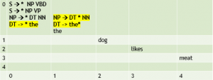
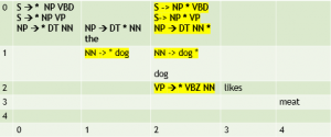
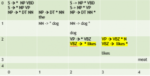
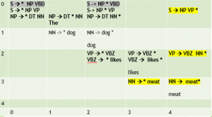
Figure A.3. A small CFG for parsing “the dog likes meat”.
`S → NP VBD S → NP VP NP → DT NN VP → VBZ NN`	`NN → dog \| meat VBD → barked VBZ → likes DT → the`

Figure A.4 shows a trace of a top-down chart parse of the sentence “The dog likes meat.”, showing the edges created in the top-down chart parser implemented in NLTK. The parse begins with top-down predictions, based on the grammar, and then begins to process the actual input, which is shown in the third row. As each word is read, there is a top-down prediction followed by an application of the fundamental rule. After an edge is completed (such as the first NP) then new predictions are added (e.g., for an upcoming VP).

Figure A.4. Trace of a top-down chart parse of the sentence “The dog likes meat.”
	[0:0] S → * NP VBD [0:0] S → * NP VP	For each of the sentence rules, make a top-down prediction to create an empty, active edge.
	[0:0] S → * NP VBD [0:0] S → * NP VP [0:0] NP → * DT NN	Make more top-down predictions to create active edges for each of the nonterminal categories just to the right of the dot.
	[0:0] S → * NP VBD [0:0] S → * NP VP [0:0] NP → * DT NN [0:0] DT → * the [0:1] DT → the * [0:1] NP → *DT NN**	Predict the and use the fundamental rule to create new edges where the dot in the DT rule and in NP rule move to the right.
	[0:0] S → * NP VBD [0:0] S → * NP VP [0:0] NP → * DT NN [0:0] DT → * the [0:1] DT → the * [0:1] NP → *DT NN [1:1] NN** → * dog [1:2] NN → dog * [0:2] NP → DT NN * [0:2] S → *NP VBD [0:2] S → NP * VP [2:2] VP** → * VBZ NN	Predict dog; apply fundamental rule and then make a top down prediction for a VP (using the second S rule.)
	[0:0] S → * NP VBD [0:0] S → * NP VP [0:0] NP → * DT NN [0:0] DT → * the [0:1] DT → the * [0:1] NP → *DT NN [1:1] NN** → * dog [1:2] NN → dog * [0:2] NP → DT NN * [0:2] S → *NP VBD [0:2] S → NP * VP [2:2] VP** → * VBZ NN [2:2] VBZ → * likes [2:3] VBZ → likes * [2:3] VP → *VBZ NN**	Predict likes; apply the fundamental rule to create VBZ-> likes , and again, to add VP -> VBZ NN
	[0:0] S → * NP VBD [0:0] S → * NP VP [0:0] NP → * DT NN [0:0] DT → * the [0:1] DT → the * [0:1] NP → *DT NN [1:1] NN** → * dog [1:2] NN → dog * [0:2] NP → DT NN * [0:2] S → *NP VBD [0:2] S → NP * VP [2:2] VP** → * VBZ NN [2:2] VBZ → * likes [2:3] VBZ → likes * [2:3] VP → *VBZ NN [3:3] NN** → * meat [3:4] NN → meat* [2:4] VP → VBZ NN * [0:4] S → NP VP *	Predict meat apply the fundamental rule for meat as a noun (NN) and again to extend the active VP edge, to get VP -> VBZ NN *. Finally, use the fundamental rule to extend the active S edge, which is now complete.

Bottom-up chart parsing algorithms, as we discussed in Chapter 4, do have some advantages. For example, bottom-up methods can use rules annotated with probabilities or semantics, and then propagate values up from the leaf to the root for each subtree. ↵

License

Icon for the Creative Commons Attribution-NonCommercial 4.0 International License

License

Share This Book