Chapter 21 Section 21.5: Exoplanets Everywhere: What We Are Learning
21.5 Exoplanets Everywhere: What We Are Learning
Learning Objectives
By the end of this section, you will be able to:
- Explain what we have learned from our discovery of exoplanets
- Identify which kind of exoplanets appear to be the most common in the Galaxy
- Discuss the kinds of planetary systems we are finding around other stars
Before the discovery of exoplanets, most astronomers expected that other planetary systems would be much like our own—planets following roughly circular orbits, with the most massive planets several AU from their parent star. Such systems do exist in large numbers, but many exoplanets and planetary systems are very different from those in our solar system. Another surprise is the existence of whole classes of exoplanets that we simply don’t have in our solar system: planets with masses between the mass of Earth and Neptune, and planets that are several times more massive than Jupiter.
Kepler Results
The Kepler telescope has been responsible for the discovery of most exoplanets, especially at smaller sizes, as illustrated in Figure 1, where the Kepler discoveries are plotted in yellow. You can see the wide range of sizes, including planets substantially larger than Jupiter and smaller than Earth. The absence of Kepler-discovered exoplanets with orbital periods longer than a few hundred days is a consequence of the 4-year lifetime of the mission. (Remember that three evenly spaced transits must be observed to register a discovery.) At the smaller sizes, the absence of planets much smaller than one earth radius is due to the difficulty of detecting transits by very small planets. In effect, the “discovery space” for Kepler was limited to planets with orbital periods less than 400 days and sizes larger than Mars.
Exoplanet Discoveries through 2017.
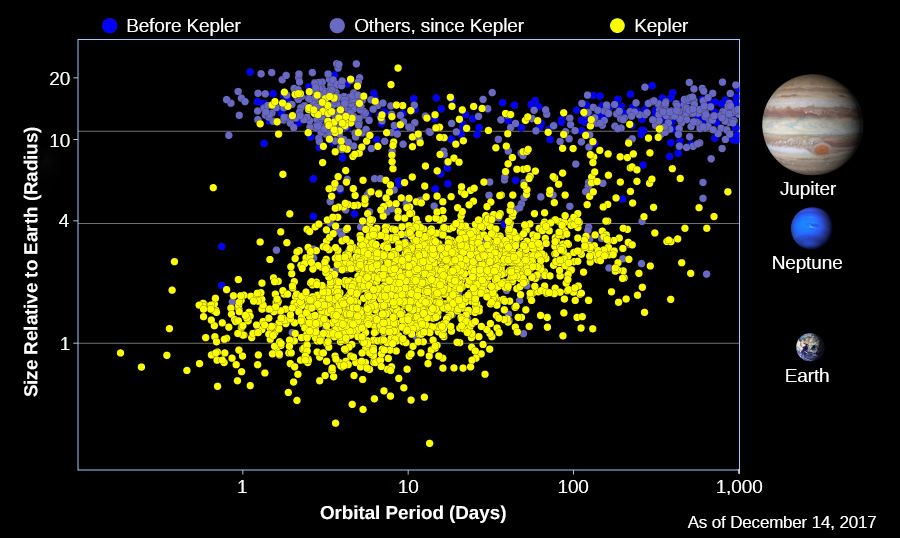
Figure 1. Exoplanet Discoveries through 2017. The vertical axis shows the radius of each planet compared to Earth. Horizontal lines show the size of Earth, Neptune, and Jupiter. The horizontal axis shows the time each planet takes to make one orbit (and is given in Earth days). Recall that Mercury takes 88 days and Earth takes a little more than 365 days to orbit the Sun. The yellow dots show planets discovered by the Kepler mission using transits, and the blue dots are the discoveries by other projects and techniques. When this graph was made, astronomers had discovered just over 3,500 exoplanets; as of the start of 2022, that number has risen to roughly 5,000. (credit: modification of work by NASA/Ames Research Center/Jessie Dotson and Wendy Stenzel)
One of the primary objectives of the Kepler mission was to find out how many stars hosted planets and especially to estimate the frequency of earthlike planets. Although Kepler looked at only a very tiny fraction of the stars in the Galaxy, the sample size was large enough to draw some interesting conclusions. While the observations apply only to the stars observed by Kepler, those stars are reasonably representative, and so astronomers can extrapolate to the entire Galaxy.
Figure 2 shows that the Kepler discoveries include many rocky, Earth-size planets, far more than Jupiter-size gas planets. This immediately tells us that the initial Doppler discovery of many hot Jupiters was a biased sample, in effect, finding the odd planetary systems because they were the easiest to detect. However, there is one huge difference between this observed size distribution and that of planets in our solar system. The most common planets have radii between 1.4 and 2.8 that of Earth, sizes for which we have no examples in the solar system. These have been nicknamed super-Earths, while the other large group with sizes between 2.8 and 4 that of Earth are often called mini-Neptunes.
Kepler Discoveries.
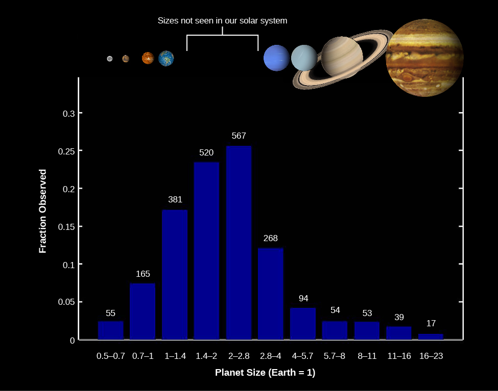
Figure 2. This bar graph shows the number of planets of each size range found among the first 2213 Kepler planet discoveries. Sizes range from half the size of Earth to 20 times that of Earth. On the vertical axis, you can see the fraction that each size range makes up of the total. Note that planets that are between 1.4 and 4 times the size of Earth make up the largest fractions, yet this size range is not represented among the planets in our solar system. (credit: modification of work by NASA/Kepler mission)
What a remarkable discovery it is that the most common types of planets in the Galaxy are completely absent from our solar system and were unknown until Kepler’s survey. However, recall that really small planets were difficult for the Kepler instruments to find. So, to estimate the frequency of Earth-size exoplanets, we need to correct for this sampling bias. The result is the corrected size distribution shown in Figure 2. Notice that in this graph, we have also taken the step of showing not the number of Kepler detections but the average number of planets per star for solar-type stars (spectral types F, G, and K).
Size Distribution of Planets for Stars Similar to the Sun.
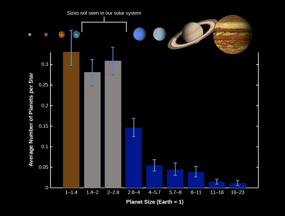
Figure 3. We show the average number of planets per star in each planet size range. (The average is less than one because some stars will have zero planets of that size range.) This distribution, corrected for biases in the Kepler data, shows that Earth-size planets may actually be the most common type of exoplanets. (credit: modification of work by NASA/Kepler mission)
We see that the most common planet sizes of are those with radii from 1 to 3 times that of Earth—what we have called “Earths” and “super-Earths.” Each group occurs in about one-third to one-quarter of stars. In other words, if we group these sizes together, we can conclude there is nearly one such planet per star! And remember, this census includes primarily planets with orbital periods less than 2 years. We do not yet know how many undiscovered planets might exist at larger distances from their star.
To estimate the number of Earth-size planets in our Galaxy, we need to remember that there are approximately 100 billion stars of spectral types F, G, and K. Therefore, we estimate that there are about 30 billion Earth-size planets in our Galaxy. If we include the super-Earths too, then there could be one hundred billion in the whole Galaxy. This idea—that planets of roughly Earth’s size are so numerous—is surely one of the most important discoveries of modern astronomy.
Planets with Known Densities
For several hundred exoplanets, we have been able to measure both the size of the planet from transit data and its mass from Doppler data, yielding an estimate of its density. Comparing the average density of exoplanets to the density of planets in our solar system helps us understand whether they are rocky or gaseous in nature. This has been particularly important for understanding the structure of the new categories of super-Earths and mini-Neptunes with masses between 3–10 times the mass of Earth. A key observation so far is that planets that are more than 10 times the mass of Earth have substantial gaseous envelopes (like Uranus and Neptune) whereas lower-mass planets are predominately rocky in nature (like the terrestrial planets).
Figure 4 compares all the exoplanets that have both mass and radius measurements. The dependence of the radius on planet mass is also shown for a few illustrative cases—hypothetical planets made of pure iron, rock, water, or hydrogen.
Exoplanets with Known Densities.
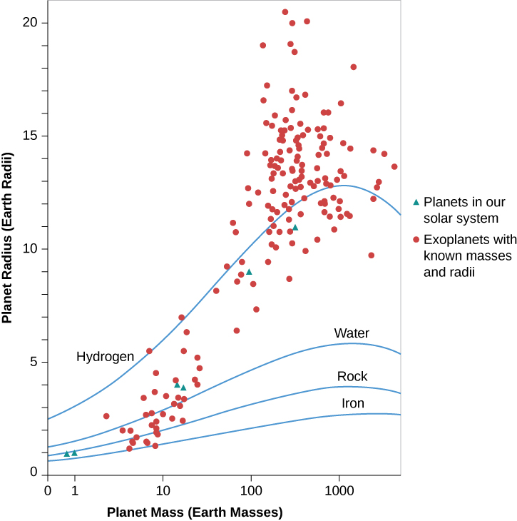
Figure 4. Exoplanets with known masses and radii (red circles) are plotted along with solid lines that show the theoretical size of pure iron, rock, water, and hydrogen planets with increasing mass. Masses are given in multiples of Earth’s mass. (For comparison, Jupiter contains enough mass to make 320 Earths.) The green triangles indicate planets in our solar system.
At lower masses, notice that as the mass of these hypothetical planets increases, the radius also increases. That makes sense—if you were building a model of a planet out of clay, your toy planet would increase in size as you added more clay. However, for the highest mass planets (M > 1000 MEarth) in Figure 4, notice that the radius stops increasing and the planets with greater mass are actually smaller. This occurs because increasing the mass also increases the gravity of the planet, so that compressible materials (even rock is compressible) will become more tightly packed, shrinking the size of the more massive planet.
In reality, planets are not pure compositions like the hypothetical water or iron planet. Earth is composed of a solid iron core, an outer liquid-iron core, a rocky mantle and crust, and a relatively thin atmospheric layer. Exoplanets are similarly likely to be differentiated into compositional layers. The theoretical lines in Figure 4 are simply guides that suggest a range of possible compositions.
Astronomers who work on the complex modeling of the interiors of rocky planets make the simplifying assumption that the planet consists of two or three layers. This is not perfect, but it is a reasonable approximation and another good example of how science works. Often, the first step in understanding something new is to narrow down the range of possibilities. This sets the stage for refining and deepening our knowledge. In Figure 4, the two green triangles with roughly 1 MEarth and 1 REarth represent Venus and Earth. Notice that these planets fall between the models for a pure iron and a pure rock planet, consistent with what we would expect for the known mixed-chemical composition of Venus and Earth.
In the case of gaseous planets, the situation is more complex. Hydrogen is the lightest element in the periodic table, yet many of the detected exoplanets in Figure 4 with masses greater than 100 MEarth have radii that suggest they are lower in density than a pure hydrogen planet. Hydrogen is the lightest element, so what is happening here? Why do some gas giant planets have inflated radii that are larger than the fictitious pure hydrogen planet? Many of these planets reside in short-period orbits close to the host star where they intercept a significant amount of radiated energy. If this energy is trapped deep in the planet atmosphere, it can cause the planet to expand.
Planets that orbit close to their host stars in slightly eccentric orbits have another source of energy: the star will raise tides in these planets that tend to circularize the orbits. This process also results in tidal dissipation of energy that can inflate the atmosphere. It would be interesting to measure the size of gas giant planets in wider orbits where the planets should be cooler—the expectation is that unless they are very young, these cooler gas giant exoplanets (sometimes called “cold Jupiters”) should not be inflated. But we don’t yet have data on these more distant exoplanets.
Exoplanetary Systems
As we search for exoplanets, we don’t expect to find only one planet per star. Our solar system has eight major planets, half a dozen dwarf planets, and millions of smaller objects orbiting the Sun. The evidence we have of planetary systems in formation also suggest that they are likely to produce multi-planet systems.
The first planetary system was found around the star Upsilon Andromedae in 1999 using the Doppler method, and many others have been found since then (about 2600 as of 2016). If such exoplanetary system are common, let’s consider which systems we expect to find in the Kepler transit data.
A planet will transit its star only if Earth lies in the plane of the planet’s orbit. If the planets in other systems do not have orbits in the same plane, we are unlikely to see multiple transiting objects. Also, as we have noted before, Kepler was sensitive only to planets with orbital periods less than about 4 years. What we expect from Kepler data, then, is evidence of coplanar planetary systems confined to what would be the realm of the terrestrial planets in our solar system.
By 2018, astronomers gathered data on nearly 3000 such exoplanet systems. Many have only two known planets, but a few have as many as five, and one has eight (the same number of planets as our own solar system). For the most part, these are very compact systems with most of their planets closer to their star than Mercury is to the Sun. The figure below shows one of the largest exoplanet systems: that of the star called Kepler-62 (Figure 5). Our solar system is shown to the same scale, for comparison (note that the Kepler-62 planets are drawn with artistic license; we have no detailed images of any exoplanets).
Exoplanet System Kepler-62, with the Solar System Shown to the Same Scale.
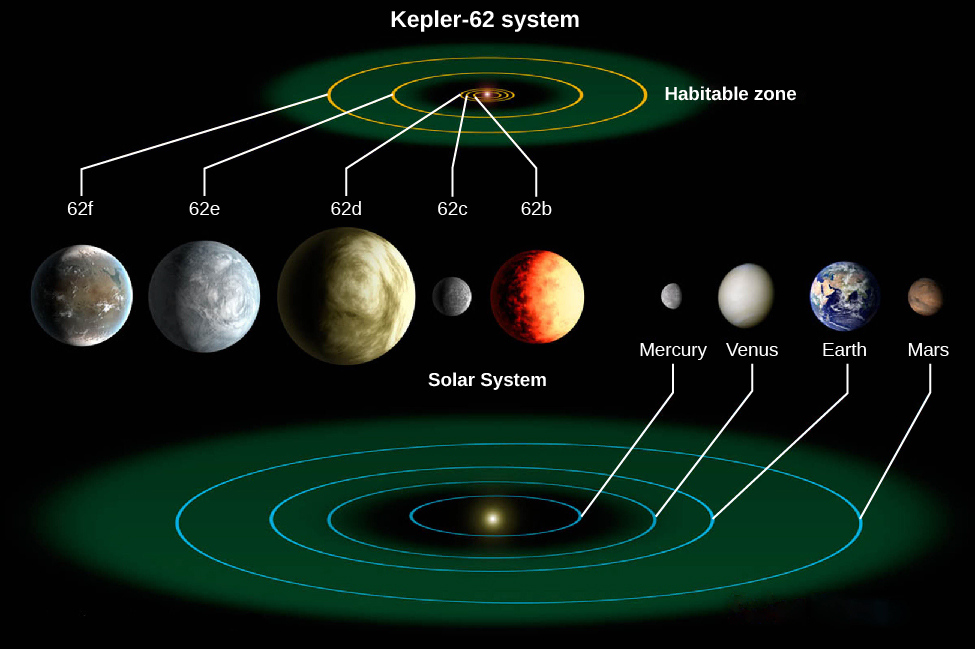
Figure 5. The green areas are the “habitable zones,” the range of distance from the star where surface temperatures are likely to be consistent with liquid water. (credit: modification of work by NASA/Ames/JPL-Caltech)
All but one of the planets in the K-62 system are larger than Earth. These are super-Earths, and one of them (62d) is in the size range of a mini-Neptune, where it is likely to be largely gaseous. The smallest planet in this system is about the size of Mars. The three inner planets orbit very close to their star, and only the outer two have orbits larger than Mercury in our system. The green areas represent each star’s “habitable zone,” which is the distance from the star where we calculate that surface temperatures would be consistent with liquid water. The Kepler-62 habitable zone is much smaller than that of the Sun because the star is intrinsically fainter.
With closely spaced systems like this, the planets can interact gravitationally with each other. The result is that the observed transits occur a few minutes earlier or later than would be predicted from simple orbits. These gravitational interactions have allowed the Kepler scientists to calculate masses for the planets, providing another way to learn about exoplanets.
Kepler has discovered some interesting and unusual planetary systems. For example, most astronomers expected planets to be limited to single stars. But we have found planets orbiting close double stars, so that the planet would see two suns in its sky, like those of the fictional planet Tatooine in the Star Wars films. At the opposite extreme, planets can orbit one star of a wide, double-star system without major interference from the second star.
Key Concepts and Summary
Although the Kepler mission is finding thousands of new exoplanets, these are limited to orbital periods of less than 400 days and sizes larger than Mars. Still, we can use the Kepler discoveries to extrapolate the distribution of planets in our Galaxy. The data so far imply that planets like Earth are the most common type of planet, and that there may be 100 billion Earth-size planets around Sun-like stars in the Galaxy. About 2600 planetary systems have been discovered around other stars. In many of them, planets are arranged differently than in our solar system.
Glossary
- super-Earth
- a planet larger than Earth, generally between 1.4 and 2.8 times the size of our planet
- mini-Neptune
- a planet that is intermediate between the largest terrestrial planet in our solar system (Earth) and the smallest jovian planet (Neptune); generally, mini-Neptunes have sizes between 2.8 and 4 times Earth’s size
For Further Exploration
Articles
Star Formation
Blaes, O. “A Universe of Disks.” Scientific American (October 2004): 48. On accretion disks and jets around young stars and black holes.
Croswell, K. “The Dust Belt Next Door [Tau Ceti].” Scientific American (January 2015): 24. Short intro to recent observations of planets and a wide dust belt.
Frank, A. “Starmaker: The New Story of Stellar Birth.” Astronomy (July 1996): 52.
Jayawardhana, R. “Spying on Stellar Nurseries.” Astronomy (November 1998): 62. On protoplanetary disks.
O’Dell, C. R. “Exploring the Orion Nebula.” Sky & Telescope (December 1994): 20. Good review with Hubble results.
Ray, T. “Fountains of Youth: Early Days in the Life of a Star.” Scientific American (August 2000): 42. On outflows from young stars.
Young, E. “Cloudy with a Chance of Stars.” Scientific American (February 2010): 34. On how clouds of interstellar matter turn into star systems.
Young, Monica “Making Massive Stars.” Sky & Telescope (October 2015): 24. Models and observations on how the most massive stars form.
Exoplanets
Billings, L. “In Search of Alien Jupiters.” Scientific American (August 2015): 40–47. The race to image jovian planets with current instruments and why a direct image of a terrestrial planet is still in the future.
Heller, R. “Better Than Earth.” Scientific American (January 2015): 32–39. What kinds of planets may be habitable; super-Earths and jovian planet moons should also be considered.
Laughlin, G. “How Worlds Get Out of Whack.” Sky & Telescope (May 2013): 26. On how planets can migrate from the places they form in a star system.
Marcy, G. “The New Search for Distant Planets.” Astronomy (October 2006): 30. Fine brief overview. (The same issue has a dramatic fold-out visual atlas of extrasolar planets, from that era.)
Redd, N. “Why Haven’t We Found Another Earth?” Astronomy (February 2016): 25. Looking for terrestrial planets in the habitable zone with evidence of life.
Seager, S. “Exoplanets Everywhere.” Sky & Telescope (August 2013): 18. An excellent discussion of some of the frequently asked questions about the nature and arrangement of planets out there.
Seager, S. “The Hunt for Super-Earths.” Sky & Telescope (October 2010): 30. The search for planets that are up to 10 times the mass of Earth and what they can teach us.
Villard, R. “Hunting for Earthlike Planets.” Astronomy (April 2011): 28. How we expect to find and characterize super-Earth (planets somewhat bigger than ours) using new instruments and techniques that could show us what their atmospheres are made of.
Websites
Exoplanet Exploration: http://planetquest.jpl.nasa.gov/. PlanetQuest (from the Navigator Program at the Jet Propulsion Lab) is probably the best site for students and beginners, with introductory materials and nice illustrations; it focuses mostly on NASA work and missions.
Exoplanets: http://www.planetary.org/exoplanets/. Planetary Society’s exoplanets pages with a dynamic catalog of planets found and good explanations.
Exoplanets: The Search for Planets beyond Our Solar System: http://www.iop.org/publications/iop/2010/page_42551.html. From the British Institute of Physics in 2010.
Extrasolar Planets Encyclopedia: http://exoplanet.eu/. Maintained by Jean Schneider of the Paris Observatory, has the largest catalog of planet discoveries and useful background material (some of it more technical).
Formation of Stars: https://www.spacetelescope.org/science/formation_of_stars/. Star Formation page from the Hubble Space Telescope, with links to images and information.
Proxima Centauri Planet Discovery: http://www.eso.org/public/news/eso1629/.
Videos
Are We Alone: An Evening Dialogue with the Kepler Mission Leaders: http://www.youtube.com/watch?v=O7ItAXfl0Lw. A non-technical panel discussion on Kepler results and ideas about planet formation with Bill Borucki, Natalie Batalha, and Gibor Basri (moderated by Andrew Fraknoi) at the University of California, Berkeley (2:07:01).
Finding the Next Earth: The Latest Results from Kepler: https://www.youtube.com/watch?v=ZbijeR_AALo. Natalie Batalha (San Jose State University & NASA Ames) public talk in the Silicon Valley Astronomy Lecture Series (1:28:38).
From Hot Jupiters to Habitable Worlds: https://vimeo.com/37696087 (Part 1) and https://vimeo.com/37700700 (Part 2). Debra Fischer (Yale University) public talk in Hawaii sponsored by the Keck Observatory (15:20 Part 1, 21:32 Part 2).
Search for Habitable Exoplanets: http://www.youtube.com/watch?v=RLWb_T9yaDU. Sara Seeger (MIT) public talk at the SETI Institute, with Kepler results (1:10:35).
Collaborative Group Activities
- Your group is a subcommittee of scientists examining whether any of the “hot Jupiters” (giant planets closer to their stars than Mercury is to the Sun) could have life on or near them. Can you come up with places on, in, or near such planets where life could develop or where some forms of life might survive?
- A wealthy couple (who are alumni of your college or university and love babies) leaves the astronomy program several million dollars in their will, to spend in the best way possible to search for “infant stars in our section of the Galaxy.” Your group has been assigned the task of advising the dean on how best to spend the money. What kind of instruments and search programs would you recommend, and why?
- Some people consider the discovery of any planets (even hot Jupiters) around other stars one of the most important events in the history of astronomical research. Some astronomers have been surprised that the public is not more excited about the planet discoveries. One reason that has been suggested for this lack of public surprise and excitement is that science fiction stories have long prepared us for there being planets around other stars. (The Starship Enterprise on the 1960s Star Trek TV series found some in just about every weekly episode.) What does your group think? Did you know about the discovery of planets around other stars before taking this course? Do you consider it exciting? Were you surprised to hear about it? Are science fiction movies and books good or bad tools for astronomy education in general, do you think?
- What if future space instruments reveal an earthlike exoplanet with significant amounts of oxygen and methane in its atmosphere? Suppose the planet and its star are 50 light-years away. What does your group suggest astronomers do next? How much effort and money would you recommend be put into finding out more about this planet and why?
- Discuss with your group the following question: which is easier to find orbiting a star with instruments we have today: a jovian planet or a proto-planetary disk? Make a list of arguments for each side of this question.
- (This activity should be done when your group has access to the internet.) Go to the page which indexes all the publicly released Hubble Space Telescope images by subject: https://hubblesite.org/resource-gallery/images. Under “Star,” go to “Protoplanetary Disk” and find a system—not mentioned in this chapter—that your group likes, and prepare a short report to the class about why you find it interesting. Then, under “Nebula,” go to “Emission” and find a region of star formation not mentioned in this chapter, and prepare a short report to the class about what you find interesting about it.
- There is a “citizen science” website called Planet Hunters (http://www.planethunters.org/) where you can participate in identifying exoplanets from the data that Kepler provided. Your group should access the site, work together to use it, and classify two light curves. Report back to the class on what you have done.
- Yuri Milner, a Russian-American billionaire, recently pledged $100 million to develop the technology to send many miniaturized probes to a star in the Alpha Centauri triple star system (which includes Proxima Centauri, the nearest star to us, now known to have at least one planet.) Each tiny probe will be propelled by powerful lasers at 20% the speed of light, in the hope that one or more might arrive safely and be able to send back information about what it’s like there. Your group should search online for more information about this project (called “Breakthrough: Starshot”) and discuss your reactions to this project. Give specific reasons for your arguments.
Review Questions
Give several reasons the Orion molecular cloud is such a useful “laboratory” for studying the stages of star formation.
Why is star formation more likely to occur in cold molecular clouds than in regions where the temperature of the interstellar medium is several hundred thousand degrees?
Why have we learned a lot about star formation since the invention of detectors sensitive to infrared radiation?
Describe what happens when a star forms. Begin with a dense core of material in a molecular cloud and trace the evolution up to the time the newly formed star reaches the main sequence.
Describe how the T Tauri star stage in the life of a low-mass star can lead to the formation of a Herbig-Haro (H-H) object.
Look at the four stages shown in this figure. In which stage(s) can we see the star in visible light? In infrared radiation?
The evolutionary track for a star of 1 solar mass remains nearly vertical in the H–R diagram for a while (see this figure). How is its luminosity changing during this time? Its temperature? Its radius?
Two protostars, one 10 times the mass of the Sun and one half the mass of the Sun are born at the same time in a molecular cloud. Which one will be first to reach the main sequence stage, where it is stable and getting energy from fusion?
Compare the scale (size) of a typical dusty disk around a forming star with the scale of our solar system.
Why is it so hard to see planets around other stars and so easy to see them around our own?
Why did it take astronomers until 1995 to discover the first exoplanet orbiting another star like the Sun?
Which types of planets are most easily detected by Doppler measurements? By transits?
List three ways in which the exoplanets we have detected have been found to be different from planets in our solar system.
List any similarities between discovered exoplanets and planets in our solar system.
What revisions to the theory of planet formation have astronomers had to make as a result of the discovery of exoplanets?
Why are young Jupiters easier to see with direct imaging than old Jupiters?
Thought Questions
A friend of yours who did not do well in her astronomy class tells you that she believes all stars are old and none could possibly be born today. What arguments would you use to persuade her that stars are being born somewhere in the Galaxy during your lifetime?
Observations suggest that it takes more than 3 million years for the dust to begin clearing out of the inner regions of the disks surrounding protostars. Suppose this is the minimum time required to form a planet. Would you expect to find a planet around a 10-MSun star? (Refer to this figure.)
Suppose you wanted to observe a planet around another star with direct imaging. Would you try to observe in visible light or in the infrared? Why? Would the planet be easier to see if it were at 1 AU or 5 AU from its star?
Why were giant planets close to their stars the first ones to be discovered? Why has the same technique not been used yet to discover giant planets at the distance of Saturn?
Exoplanets in eccentric orbits experience large temperature swings during their orbits. Suppose you had to plan for a mission to such a planet. Based on Kepler’s second law, does the planet spend more time closer or farther from the star? Explain.
Figuring for Yourself
When astronomers found the first giant planets with orbits of only a few days, they did not know whether those planets were gaseous and liquid like Jupiter or rocky like Mercury. The observations of HD 209458 settled this question because observations of the transit of the star by this planet made it possible to determine the radius of the planet. Use the data given in the text to estimate the density of this planet, and then use that information to explain why it must be a gas giant.
An exoplanetary system has two known planets. Planet X orbits in 290 days and Planet Y orbits in 145 days. Which planet is closest to its host star? If the star has the same mass as the Sun, what is the semi-major axis of the orbits for Planets X and Y?
Kepler’s third law says that the orbital period (in years) is proportional to the square root of the cube of the mean distance (in AU) from the Sun (P ∝ a1.5). For mean distances from 0.1 to 32 AU, calculate and plot a curve showing the expected Keplerian period. For each planet in our solar system, look up the mean distance from the Sun in AU and the orbital period in years and overplot these data on the theoretical Keplerian curve.
Calculate the transit depth for an M dwarf star that is 0.3 times the radius of the Sun with a gas giant planet the size of Jupiter.
If a transit depth of 0.00001 can be detected with the Kepler spacecraft, what is the smallest planet that could be detected around a 0.3 Rsun M dwarf star?
What fraction of gas giant planets seems to have inflated radii?
